Bergman

Introduction

Figure 1: LiDAR systems capture sparse 3D point clouds with high accuracy (bottom). A high-resolution RGB image (top) can be processed with a monocular depth estimation algorithm to compute an initial estimate of a dense depth map of the scene (second row), but depth predictions from monocular images contain ambiguity and are not accurate. We propose an adaptive sampling method which is guided by the RGB image and a depth completion network to resolve these ambiguities. Our method (third row) computes dense depth maps with a significantly higher quality than monocular depth estimators and additionally provides the sparse sample locations which result in the best possible inpainted depth images. Note that the ground truth image is also sparse in this figure - however it is far more dense than the sampling densities that we use for reconstruction. RMSE of the predicted dense depth estimated is calculated against the ground truth depth image at points that have defined depth, and is listed in millimeters. Red regions of the image correspond to higher depths, while blue regions of the image correspond to shallower depths. In the ground truth depth image, the dark blue background corresponds to 0 depth, or a missing depth value.

Imaging systems using active illumination and time-resolved detectors are able to make precise depth measurements guided by their own light sources. This capability of capturing 3D information is useful for applications such as autonomous vehicle navigation and robotics [1] and remote sensing [2]. With advances in imaging hardware and processing algorithms, light detection and ranging (LiDAR) systems can capture depth images at extremely long range [3], high speed [4], or high resolution. However, there exists a trade-off between these advances to obtain depth images without sacrificing accuracy. One way to address this trade-off is through depth completion, where dense depth is predicted from a sparse set of initial samples and a single RGB image. This removes the requirement to densely scan a scene for high resolution depth images, requiring a significant amount of time. Recent results in depth completion [5-9] have shown promising results on this task, but performance typically degrades sharply for very low depth sampling rates. This intuitively makes sense, since low sampling rates of high frequency details in the depth image prevent perfect reconstruction as governed by the Nyquist-Shannon sampling theorem. Methods using deep learning for depth completion [5-9] can attempt to hallucinate these details, but performance still degrades with low numbers of samples.

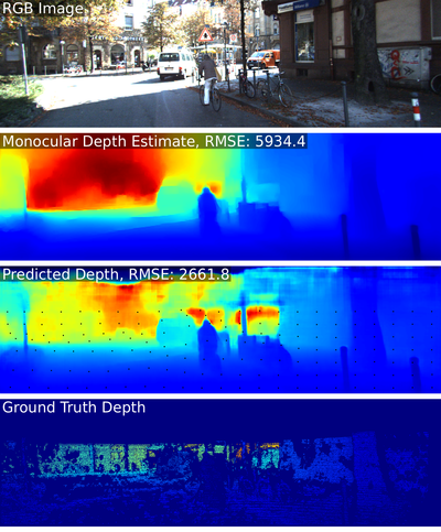
In this project, we propose an imaging system which obtains dense depth maps from an RGB image and sparse depth measurements generated by a scene-adaptive scanning pattern. Our method is based on a novel deep neural network architecture for solving the depth completion task, and a deep learning architecture for predicting the sampling locations, which can be trained in an end-to-end fashion. An outline of the results of this system is shown in Figure 1. We show that exploiting adaptive sampling by predicting depth sampling locations from an RGB image improves performance of depth completion networks, especially at low sampling rates.

Background

3D Imaging

Our method is partially motivated by improvements in scanning LiDAR and emerging optical phased array imaging systems [10]. These phased array imaging systems have the unique capability of rapidly generating arbitrary scan patterns and could facilitate the implementation of adaptive sampling algorithms in 3D imaging applications. This is because our adaptive sampling system is designed with the idea that our system could take arbitrary scan patterns at no additional resolution, speed, or range cost, and phased array imaging systems meet this criterion. Note that for traditional scanning LiDAR systems, solely based on the time-of-flight of light alone, in order to take measurements at 200 meters, 750 measurements could take up to 1 millisecond. This is not including the time required to steer the laser to each of these points. Thus, this work opens discussion of the discussion of the development of adaptive sampling algorithms which are sure to become important as imaging systems advance in this direction.

Depth Estimation

Early methods in monocular depth estimation used hand-crafted features and graphical models [11] to map monocular images to depth given a large repository of RGB-depth data. Since the success of deep learning and convolutional neural networks (CNNs), these tools have been used to directly learn a mapping from monocular images to dense depth [12]. However, due to the ambiguity of absolute depth values in estimation from monocular images, these methods struggle in producing accurate depth estimates. Often times, the resulting estimated depth is off by a scale and bias factor, i.e. these methods produce accurate ordinal depth and edges, but not accurate depth values.

The depth completion task was proposed to help resolve some of the ambiguities in monocular depth estimation by fusing a monocular image and a few sparse depth samples to predict a dense depth images. The reasoning behind this was that if the monocular depth images were off by a scale and bias factor, the few sparse depth samples would be enough to anchor the absolute depth values and produce both accurate ordinal depth and actual depth values. The advent of deep learning brought upon numerous CNN modifications and architectures designed to predict dense depth on this depth completion task [5-9]. Still other non-learning based methods have used bilateral filters [14] and optimization [15] to solve the depth completion problem without requiring large datasets to train deep learning models.

Our adaptive sampling system proposed to provide generalization one step further for depth estimation; now our system has the freedom to decide where to sample along with designing a depth completion system. Still, the goal of this system remains to produce the best dense depth estimate of a scene.

Adaptive Sampling

Previous approaches for predicting sample locations proposed sampling heuristics to capture the underlying image signal. For images, furthest point sampling [16] was proposed as a good heuristic to sample images for later image reconstruction. More sophisticated heuristics for progressive image sampling have been proposed based on statistical information in regions of the image or wavelets [17], and come close to adaptive sampling, but do not optimize sample locations for a specific upstream inference task such as dense depth reconstruction. Our formulation allows us to directly optimize these sampling locations using first order optimization methods in order to improve an upstream loss rather than relying on sampling patterns that we already know to be successful for various tasks.

Methods

Our method for depth completion and adaptive sampling is outlined in Figure 2. It takes as input an RGB image, and outputs a reconstructed dense depth image. This is done by determining locations to sample for depth from the RGB image, sampling those locations, and then using those sparse samples and RGB image to reconstruct a dense depth image of the scene.

Figure 2: Our adaptive sampling deep network takes as input an RGB image, and predicts optimal sampling pattern and reconstructed dense depth from sampling at these locations. A pre-trained monocular depth estimation network is used to make an initial dense depth estimate of the scene from the RGB image, essentially pre-processing that image. A U-Net is used to extract a sampling importance vector field from the monocular depth estimate. This vector field is integrated in order to decide the locations to sample in this scene. The depth completion network fuses together the coarsely inpainted sparse depth samples with the monocular depth estimate and predicts a final dense depth. The example image is from the NYU-Depth-v2 dataset [18]

Preprocessing & Depth Completion

We have observed that many depth completion networks perform much worse with a low number of sparse samples. Prior work [13] has shown that traditional convolution kernels used in CNNs are not well suited for sparse images. Additionally, as we can observe in the comparison results figures, many depth completion networks blur the high frequency details in the depth image such as the boundaries between objects in the depth domain. This results in depth images which are accurate in the MSE sense, but since this loss function doesn't necessarily represent perception and edges well, then the network learns to disregard these details. This is in contrast to many monocular depth estimation networks which attempt to reconstruct depth from only an RGB image. Since these networks are generally trained using SSIM losses or losses on the gradient of the depth images (corresponding to the edges in the depth domain), these networks produce depth images which capture high frequency details well.

Based on these observations, we propose preprocessing the RGB data with a monocular depth estimation network to predict a dense depth map from the input RGB image. This way, we input to our depth completion network an image in the depth domain which accurately captures high frequency edge details. This is shown in Figure 2 as the monocular depth estimation network. We also use a bilateral filter to roughly inpaint the captured sparse depth image, shown in the bilateral filter block of Figure 2. This gets around the problematic sparse images inputted into the neural network, as it estimates a depth value for every pixel. Additionally, we tune the bilateral filter inpainting in such a way that it does not capture high frequency details in the depth domain and instead just blurs the sparse depth out with minor edge awareness. With these two inputs to our depth completion network, our network only needs to learn to apply a high pass filter to the monocular depth estimate and a low pass filter to the bilateral inpainted sparse depth. Additionally, since both images are in the depth domain, we expect our network to have an easier time learning a mapping to dense depth images than if we had fused RGB images with sparse depth like many other depth completion networks do.

For the depth completion network itself, we use an early fusion architecture, meaning that the inputs are concatenated together at the input of the network without gone through deep learning blocks to learn features independently. For the KITTI dataset, we use the fusion network proposed in [9], which is based on ResNet-34 [21] and also has 4 down-sampling and up-sampling residual blocks. This architecture is referred to as the depth completion network in Figure 2.

Sample Prediction and Differentiable Sampling

From previous experiments and literature, we found that furthest point sampling (i.e. spreading the sampling locations as far apart as possible in the scene) consistently outperforms random sampling on the depth completion task. The implementation of furthest point sampling that we use is that of Poisson-disc sampling [22], which produces a set of sampling points which are tightly packed but no closer than a minimum distance $r$. Because of this observation, we propose to perform adaptive sampling by beginning with our sampling locations on a grid of points spaced as far apart as possible, and then predict how much to move each of these points away from their original grid formation. With regularization on the movement of the samples, we can use this initial grid based sampling pattern as a prior.

To predict how much to move each of these sampling locations, we use a deep neural network (U-Net with 4 down- and up-sampling layers) which takes in the monocular depth estimate image and outputs a sampling importance flow field. This vector flow field allows the network to learn which regions of the image are important to place more samples into, and so any initial sampling pattern can modified by integrating the flow field in order to improve the resulting reconstructed image. In our case, each of the initially placed grid sampling locations integrates the vector flow field weighted by proximity of a vector to the sample, where the weights are a Gaussian function of distance. This formulation is given by:

$V_{i,j}=\sum _{u=i-H}^{i+H}\sum _{v=j-W}^{j+W}{\mathcal {G}}(u,v)\cdot V_{u,v}$

where $V_{i,j}$ is the sampling importance vector at coordinate $(i,j)$, $H$ and $W$ are the spacing of the initial grid samples in the vertical and horizontal direction respectively, and ${\mathcal {G}}$ is a 2D Gaussian function centered at $(i,j)$ with a standard deviation of $((2/3)H,(2/3)W)$.

The resulting vector from this summation dictates where the initial grid sample moves to, resulting in a new sampling pattern for the image. We train the sampling importance flow field prediction network by varying the number of the grid samples with each iteration, in order to make the resulting flow field prediction robust to the original grid sampling locations. Since this is just a summation of the values outputted in the sampling importance vector field, this new sampling location is a differentiable function of the output of the network and can thus be backpropagated through. However, in order to train the sampling importance field prediction network, we need to find a differentiable pipeline connecting the location of the sparse depth samples to the output dense depth image, which we can apply a loss to. We use the PyTorch [23] implementation of differentiable image sampling, based on that proposed in [24], in order to differentiably relate the values of the sparse points to the sampling locations. The differentiability comes from sampling the value at $(i,j)$ with a bilinear kernel, as described in the following equation where $D_{i,j}$ is the sampled depth value at $(i,j)$ and $I$ is the ground truth depth image of dimension $X\times Y$.

$D_{i,j}=\sum _{n=0}^{X}\sum _{m=0}^{Y}I_{n,m}\max(0,1-|i-n|)\max(0,1-|j-m|)$

With this formulation, gradients from the loss on our depth completion network can be backpropagated from the sparse sample values into the sampling locations of the points, which can then be used to train the sampling importance field prediction network.

Loss functions & Regularization

To encourage our network to include the high frequency details contained in the monocular depth estimate ${\hat {d}}_{m}$ and the accurate absolute depth scale present in the inpainted sparse depth image, we apply a loss to the output depth image which includes the MSE between the output predicted depth image and the ground truth depth image, and a SSIM loss between the output predicted depth image and the monocular depth estimate. The intuitive goal of the SSIM loss is to maintain the structural similarity to the monocular depth estimate in a somewhat scale-invariant way, while refining the absolute depth scale to minimize the MSE between the predicted dense depth image and the ground truth depth image. Thus, our loss function on the predicted image ${\hat {d}}$, where $d_{gt}$ is the ground truth depth image, is:

${\mathcal {L}}_{prediction}=||d_{gt}-{\hat {d}}||^{2}+0.5\cdot SSIM({\hat {d}},{\hat {d}}_{m})$

In order to use the grid based sampling as a prior, we implement a regularization on the predicted sampling importance flow field $V$ which penalizes large vectors. This intuitively corresponds to penalizing moving the samples too far from their starting grid positions, essentially defining these grid positions as a prior for the image sampling. This regularization is given by:

${\mathcal {L}}_{field}=||V||^{2}$

The final loss is given by a sum of the output loss and the regularization term, where $r_{1}$ is a weighting of the regularization term:

${\mathcal {L}}={\mathcal {L}}_{prediction}+r_{1}\cdot {\mathcal {L}}_{field}$

For our best performing networks, we used a value of $r_{1}=100$.

Implementation Details

In order to use the monocular depth estimation network as a preprocessing step, we must first train this network and then freeze its parameters while we train the sampling importance flow field prediction network and depth completion network end-to-end. In order to do this, we must split our training dataset into thirds to ensure that the pre-processing network is not operating on data that is in its training set. So, we use the first third of our dataset in order to train the monocular depth estimation network that is used as a preprocessing step for the RGB image, and we use the remaining two thirds to train the depth completion network and sampling importance flow field prediction network. For training the depth completion network and sampling importance flow field prediction, we first begin by training the depth completion network with random sampling patterns. After 15 epochs, we insert our adaptive sampling method and continue training both the depth completion network and sampling importance flow field network end-to-end.

For the bilateral filter implementation, we fit a neural network to the output of the fast bilateral solver [14] over our entire dataset. This is done because the neural network is faster to run in the forward and backward pass than the bilateral solver, which we desired. This neural network uses a canned U-Net architecture with 4 down-sampling and 4 up-sampling layers. The monocular depth estimation network was taken from [12] and trained according to the default parameters specified in that paper. Our depth completion networks were trained with a learning rate of $0.0003$ and a batch size of $12$, while our sampling importance field prediction network was trained using a learning rate of $10^{-5}$ and only using the MSE part of the loss (removing the SSIM).

In order to train the adaptive sampling networks, we expect there to be a dense ground truth depth image to sample from, since in practice we would be directly measuring these values from the scene. In the case of KITTI, however, the ground truth depth images are not dense since they are collected from a velodyne LiDAR. In order to combat this, we inpaint these ground truth depth images with the optimization based method in [15]. This gives us a plausible ground truth depth map, which we then take as ground truth in our reconstruction task. Since we only train our network and evaluate it for accuracy on the sparse ground truth points presented in the KITTI dataset, the validity of this inpainting only comes into question when training the sampling importance flow field.

Results

Adaptive Sampling

Figure 3: Comparison of various state of the art depth completion methods on the KITTI dataset. Ours outperforms all other methods at very low sampling rates, and outperforms multiple others at increasing sampling rates.

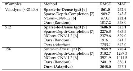
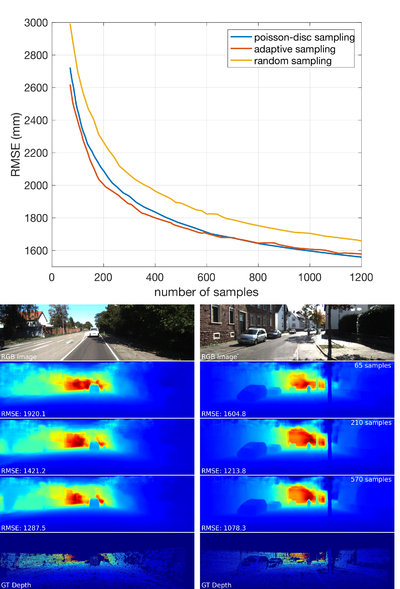
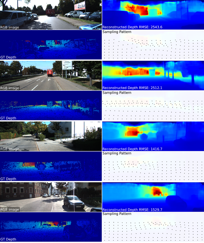
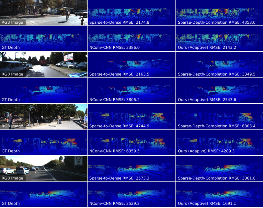
Figure 3 shows that with adaptive sampling, we improve upon our own network's performance significantly. We observe that at low sampling rates, the adaptive sampling is able to outperform state-of-the-art depth completion using random sampling. Figure 4 shows the improvement of adaptive sampling over random sampling and Poisson-disc sampling as the number of samples decreases. Here we observe that adaptive sampling consistently performs better than other sampling strategies, and the amount of performance increase increases as the number of samples decreases. However, we do observe that choosing clever heuristics for sampling such as furthest point sampling also creates greater increases in performance as the number of samples gets low. This is expected, since at lower number of samples the choice of the sampling locations becomes more important to capture all of the information in the scene. Figure 5 shows the reconstructed dense depth images and predicted sampling masks for the adaptive sampling strategy. Here, we see that the adaptive samples cluster to regions where not sampling enough would produce a large MSE loss, like the regions in the image which are furthest away, since these contribute the most to the MSE loss when they are not accurate.

Figure 4: Comparison of our method using various sampling strategies as the number of samples decreases. Note that all sampling strategies suffer from the same exponential fall-off in performance as the number of samples decreases, however, because of this our adaptive sampling method results in increasing gains as the number of samples decreases.

Qualitative comparisons of other depth completion methods with out adaptive sampling method at low sampling densities are seen in Figure 6. Here, we see that at lower sampling densities our depth images still preserve the high frequency boundaries of objects in the scene seen in the RGB images. This preservation is not observed in other depth completion methods, which blur the boundaries of depth edges in the scene.

Figure 5: Visualization of the learned sampling pattern and the reconstructed dense depth images using our method. Note that the samples cluster in regions of the depth image which correspond to far away (red). This is because getting these depth values wrong would have the largest impact on the MSE error which we are optimizing for.

Figure 6: Comparison of various depth completion methods with our adaptive sampling method at the ground truth values that were captured using the velodyne in the KITTI dataset. This figure was generated for 156 samples per image. Red regions of the image correspond to higher depths, while blue regions of the image correspond to shallower depths. In the ground truth depth image, the dark blue background corresponds to 0 depth, or a missing depth value. RMSE is measured in millimeters.

Depth Completion

We also evaluate and compare our network on the depth completion task. For this evaluation, the adaptive sampling method is replaced by generating random sampling masks with a desired number of samples. In Figure 3, we see this performance listed under Ours (Random) compared to the other state of the art methods. We see that our network is competitive versus state of the art methods even with just random sampling, and at low sampling densities out-performs many of them. For example, methods [6-7] have performance within 100mm of the top performing method for depth completion on the KITTI benchmark, but do not perform as well in the low sampling rate regime. This is because at lower numbers of samples, it is especially important to leverage the high quality ordinal depth obtained using monocular depth estimation for sensor fusion with an image generated from the sparse samples.

Conclusions

The end-to-end trainable adaptive sampling method displayed in this paper both quantitative and qualitatively shows improvement over random sampling and simple heuristics such as furthest point sampling implemented with the Poisson-disc algorithm. We believe that further improvement on the adaptive sampling task in depth completion is limited by the following challenges.

First, optimizing sampling locations directly is a fundamentally non-differentiable problem, and thus our differentiable formulations of the problem which allow us to apply first order optimization methods such as gradient descent are only an approximation of the real function which maps predicted sampling locations to predicted depth. The gradients that we use for backpropagation and optimization of the sampling importance flow field prediction network are thus only an approximation of the ones which lead to optimal parameters, which limits the accuracy to which we can train this network. Future work could involve coming up with a better approximation for this non-differentiable function, or developing a new method which doesn't depend on first order optimization methods.

Second, depth completion implemented with deep neural networks may not utilize information from samples in the way that we intuitively expect. It is possible that the mapping deep neural networks learn from RGB and sparse depth to dense depth is more invariant to the locations of the sparse samples than the human visual system is when obtaining information about a scene. This could help explain why sampling heuristics such as furthest point sampling perform so well - perhaps a regular space of points is all that dense depth reconstruction needs to be relatively accurate, and optimizing these points is bound to get instantly stuck in a local minima because there are many equally good sampling patterns. Future work could involve training the adaptive sampling for a task where the locations of the sparse samples matters much more, such as a classification or segmentation task. Perhaps in this case, we could observe sampling patterns which approach which match what we intuitively expect from our knowledge about the human visual system, such as sampling patterns which match the distribution of cones and rods in the fovea in areas that we are interested in focusing on in the image.

However, this method opens a new direction of research for developing imaging systems which are capable of actively determining where to sample and performing some inference task with these samples in an end-to-end optimized method. In this work, we present an implementation of this kind of imaging system and apply it to the case of depth imaging.

References

[1] B. Schwarz, “LIDAR: Mapping the world in 3D,” Nature Photonics, vol. 4, pp. 429–430, 2010.

[2] U. Weiss and P. Biber, “Plant detection and mapping for agricultural robots using a 3D LIDAR sensor,” Robotics and Autonomous Systems, vol. 59, pp. 265–273, 2011.

[3] A. M. Pawlikowska, A. Halimi, R. A. Lamb, and G. S. Buller, “Single-photon three-dimensional imaging at up to 10 kilometers range,” Optics Express, vol. 25, no. 10, pp. 11 919–11 931, 2017.

[4] D. B. Lindell, M. OToole, and G. Wetzstein, “Single-Photon 3D Imaging with Deep Sensor Fusion,” ACM Trans. Graph. (SIG548 GRAPH), no. 4, 2018.

[5] F. Ma and S. Karaman, “Sparse-to-dense: Depth prediction from sparse depth samples and a single image,” ICRA, 2018.

[6] A. Eldesokey, M. Felsberg, and F. Khan, “Confidence propagation through cnns for guided sparse depth regression,” IEEE PAMI, 2019.

[7] W. Van Gansbeke, D. Neven, B. De Brabandere, and L. Van Gool, “Sparse and noisy lidar completion with rgb guidance and uncertainty,” in 2019 16th International Conference on Machine Vision Applications (MVA), 2019.

[8] X. Cheng, P. Wang, and R. Yang, “Depth estimation via affinity learned with convolutional spatial propagation network,” in ECCV, 2018.

[9] F. Ma, G. V. Cavalheiro, and S. Karaman, “Self-supervised sparse-to-dense: Self-supervised depth completion from lidar and monocular camera,” ICRA, 2019.

[10] J. Sun, E. Timurdogan, A. Yaacobi, E. S. Hosseini, and M. R. Watts, “Large-scale nanophotonic phased array,” Nature, vol. 493, pp. 195–199, 2013.

[11] A. Saxena, S. H. Chung, and A. Y. Ng, “Learning depth from single monocular images,” in Advances in Neural Information Processing Systems, 2006.

[12] I. Alhashim and P. Wonka, “High quality monocular depth estimation via transfer learning,” arXiv:1812.11941, 2018.

[13] J. Uhrig, N. Schneider, L. Schneider, U. Franke, T. Brox, and A. Geiger, “Sparsity invariant cnns,” International Conference on 3D Vision (3DV), 2017.

[14] J. T. Barron and B. Poole, “The fast bilateral solver,” in ECCV, 2016.

[15] A. Levin, D. Lischinski, and Y. Weiss, “Colorization using optimization,” in ACM SIGGRAPH, 2004.

[16] Y. Eldar, M. Lindenbaum, M. Porat, and Y. Y. Zeevi, “The Farthest Point Strategy for Progressive Image Sampling,” IEEE TIP, vol. 6, no. 9, pp. 1305–1315, 1997.

[17] V. Saragadam and A. Sankaranarayanan, “Wavelet tree parsing with freeform lensing,” in IEEE ICCP, 2019.

[18] P. K. Nathan Silberman, Derek Hoiem and R. Fergus, “Indoor segmentation and support inference from rgbd images,” in ECCV, 2012.

[19] O. Ronneberger, P. Fischer, and T. Brox, “U-net: Convolutional networks for biomedical image segmentation,” arXiv:1505.04597, 2015.

[20] A. Geiger, P. Lenz, C. Stiller, and R. Urtasun, “Vision meets robotics: The KITTI dataset,” International Journal of Robotics Research (IJRR), 2013.

[21] K. He, X. Zhang, S. Ren, and J. Sun, “Deep residual learning for image recognition,” arXiv:1512.03385, 2015.

[22] R. Bridson, “Fast poisson disk sampling in arbitrary dimensions,” in ACM SIGGRAPH 2007 Sketches, ser. SIGGRAPH ’07, 2007.

[23] A. Paszke, S. Gross, S. Chintala, G. Chanan, E. Yang, Z. DeVito, Z. Lin, A. Desmaison, L. Antiga, and A. Lerer, “Automatic differentiation in PyTorch,” in NeurIPS Autodiff Workshop, 2017.

[24] M. Jaderberg, K. Simonyan, A. Zisserman, and K. Kavukcuoglu, “Spatial transformer networks,” in Advances in Neural Information Processing Systems, 2015.

Appendix

This work is a collaboration with David B. Lindell and Gordon Wetzstein of the Stanford Computational Imaging Group. The team member contribution is broken down as follows:

Alexander W. Bergman (PSYCH 221 student) performed the literature review and analysis, helped brainstorm the solution method, implemented the methods and collected the results, formulated the conclusion drawn from the results, and wrote the report.

David B. Lindell (non-PSYCH 221 student) proposed the idea for the project, helped with the literature review, provided guidance and suggestions on the methods, helped speculate on the interpretation of the results.

Gordon Wetzstein (non-PSYCH 221 student) defined the motivation for the project and desired results to pursue, helped with the literature review, provided guidance and suggestion on the methods, and provided the computing resources for developing the project.

I would like to thank my collaborators for their suggestions and guidance in my development of this project - without their input this project would not be where it is now. I'd also like to thank Professor Wandell, Zheng Lyu, and Dr. Farrell for their insightful comments during my presentation which helped guide my writing of this report.

Source Code

The repository containing the source code for the methods and evaluation of this project is available upon request. Contact awb@stanford.edu. (Don't want to make the code publicly available yet).