Simulation of Optical Response in Oral Tissue: Difference between revisions
| (19 intermediate revisions by 2 users not shown) | |||
| Line 1: | Line 1: | ||
== Introduction == | == Introduction == | ||
Oral cancer remains a significant global health challenge, where early detection is the most critical factor in improving survival rates. Traditionally, screening has relied on standard white light examinations; however, this method is limited by the human eye's error-prone ability to detect subtle lesions that may not clearly manifest under typical examinations. To address these limitations, the VELscope has emerged as a promising, non-invasive, and rapid technology for efficiently screening oral tissue. | Oral cancer remains a significant global health challenge, where early detection is the most critical factor in improving survival rates. Traditionally, screening has relied on standard white light examinations; however, this method is limited by the human eye's error-prone ability to detect subtle lesions that may not clearly manifest under typical examinations. To address these limitations, the VELscope[[#References|[8]]] has emerged as a promising, non-invasive, and rapid technology for efficiently screening oral tissue. | ||
Leading this technological shift is the VELscope, a handheld device that utilizes blue excitation light to visualize tissue abnormalities. Under VELscope illumination, healthy tissue emits a pale green fluorescence due to fluorophores such as collagen, whereas cancerous tissue typically appears as a distinct "dark spot" due to a loss of fluorescence. This contrast enhancement addresses the limitations of incandescent white light, clearly illuminating potential lesions that might otherwise go unnoticed. | <span id="Figure_1"></span> | ||
<div style="text-align:center;"> | |||
[[File:Velscope.jpg|300px|center]] | |||
</div> | |||
<div style="text-align:center;">'''Figure 1:''' The VELscope technology used for oral cancer detection.</div> | |||
Leading this technological shift is the VELscope, a handheld device that utilizes blue excitation light to visualize tissue abnormalities. Under VELscope illumination, healthy tissue emits a pale green fluorescence due to fluorophores such as collagen, whereas cancerous tissue typically appears as a distinct "dark spot" due to a loss of fluorescence[[#References|[8]]]. This contrast enhancement addresses the limitations of incandescent white light, clearly illuminating potential lesions that might otherwise go unnoticed. | |||
Despite the clinical utility of the VELscope, a significant gap remains in the interpretation of these "dark spots." While the device is effective at identifying areas of low fluorescence, it lacks specificity regarding the biological cause of the signal loss; it could simply be a concentrated blood spot. Crucially, limited research has been conducted to distinguish between dark spots caused by cancer, and those caused by benign "blood spots" resulting from trauma, infection, or inflammation. Hemoglobin is a potent absorber of light in the blue-green spectrum, and therefore increased blood volume can mimic the optical appearance of a cancerous lesion by absorbing the fluorescence before it reaches the detector. This ambiguity presents a diagnostic challenge: a "dark spot" could represent a malignant breakdown of collagen, or it could simply represent a localized accumulation of blood due to another health issue. To improve the specificity of autofluorescence screening, it is essential to decouple the optical effects of blood absorption from true tissue fluorescence. | Despite the clinical utility of the VELscope, a significant gap remains in the interpretation of these "dark spots." While the device is effective at identifying areas of low fluorescence, it lacks specificity regarding the biological cause of the signal loss; it could simply be a concentrated blood spot. Crucially, limited research has been conducted to distinguish between dark spots caused by cancer, and those caused by benign "blood spots" resulting from trauma, infection, or inflammation. Hemoglobin is a potent absorber of light in the blue-green spectrum, and therefore increased blood volume can mimic the optical appearance of a cancerous lesion by absorbing the fluorescence before it reaches the detector. This ambiguity presents a diagnostic challenge: a "dark spot" could represent a malignant breakdown of collagen, or it could simply represent a localized accumulation of blood due to another health issue. To improve the specificity of autofluorescence screening, it is essential to decouple the optical effects of blood absorption from true tissue fluorescence. | ||
In this paper, we address this challenge by simulating the optical response of oral tissue using Monte Carlo modeling in MCmatlab. Prior research, notably by Pavlova et al., has successfully employed multi-layered Monte Carlo models to predict fluorescence spectra in oral neoplasia, establishing the importance of site-specific optical properties and layered tissue geometries. However, they primarily focused on intrinsic fluorophores rather than the specific depth-dependent reflectance signatures caused by variable blood accumulation. By computationally modeling the interaction of light with varying depths of blood vessels and tissue layers -- specifically comparing the response at the highly absorbing 415 nm wavelength versus the more penetrating 450 nm wavelength -- we aim to investigate the impact of blood on tissue reflectance. This study seeks to provide a new theoretical framework for detecting benign blood absorption in oral tissue, potentially reducing false positives in optical oral cancer screening. | In this paper, we address this challenge by simulating the optical response of oral tissue using Monte Carlo modeling in MCmatlab. Prior research, notably by Pavlova et al.[[#References|[2]]], has successfully employed multi-layered Monte Carlo models to predict fluorescence spectra in oral neoplasia, establishing the importance of site-specific optical properties and layered tissue geometries. However, they primarily focused on intrinsic fluorophores rather than the specific depth-dependent reflectance signatures caused by variable blood accumulation. By computationally modeling the interaction of light with varying depths of blood vessels and tissue layers -- specifically comparing the response at the highly absorbing 415 nm wavelength versus the more penetrating 450 nm wavelength -- we aim to investigate the impact of blood on tissue reflectance. This study seeks to provide a new theoretical framework for detecting benign blood absorption in oral tissue, potentially reducing false positives in optical oral cancer screening. | ||
== Background == | == Background == | ||
| Line 53: | Line 59: | ||
</p> | </p> | ||
<p> | <p> | ||
All optical coefficients at 415 nm were taken directly from Pavlova et al.'s Monte Carlo study of oral fluorescence, which provides wavelength-specific absorption and scattering parameters for a five-layer oral tissue model | All optical coefficients at 415 nm were taken directly from Pavlova et al.'s Monte Carlo study of oral fluorescence, which provides wavelength-specific absorption and scattering parameters for a five-layer oral tissue model[[#References|[2]]]. For 450 nm, scattering coefficients were computed following the same methodology as Pavlova, using a power-law spectral dependence commonly applied to biological tissues[[#References|[4]]]. | ||
</p> | </p> | ||
<p> | <p> | ||
| Line 67: | Line 73: | ||
<p> | <p> | ||
A simple Monte Carlo simulation can be used to estimate the value of π by comparing areas of a circle and a square. First, the geometric domain is defined, consisting of a square whose side is equal to twice the radius <math>R</math> of the circle, so that the circle is fully inscribed within the square (see [[# | A simple Monte Carlo simulation can be used to estimate the value of π by comparing areas of a circle and a square. First, the geometric domain is defined, consisting of a square whose side is equal to twice the radius <math>R</math> of the circle, so that the circle is fully inscribed within the square (see [[#Figure_2|Figure 2a]]). A large number of points are then generated randomly and uniformly within the square. Each point is classified according to whether it lies inside the circle or outside, and the number of points falling within the circle is counted (see [[#Figure_2|Figure 2b]]). The ratio of the number of points inside the circle <math>N_\text{circle}</math> to the total number of points in the square <math>N_\text{total}</math> approaches the ratio of the areas of the circle and the square: | ||
<math>\frac{N_\text{circle}}{N_\text{total}} \approx \frac{\text{Area of circle}}{\text{Area of square}} = \frac{\pi R^2}{(2R)^2} = \frac{\pi}{4}</math>. | <math>\frac{N_\text{circle}}{N_\text{total}} \approx \frac{\text{Area of circle}}{\text{Area of square}} = \frac{\pi R^2}{(2R)^2} = \frac{\pi}{4}</math>. | ||
Multiplying this ratio by four therefore provides an estimate of π. This example illustrates how probabilistic sampling can be used to approximate geometric quantities. | Multiplying this ratio by four therefore provides an estimate of π. This example illustrates how probabilistic sampling can be used to approximate geometric quantities. | ||
| Line 76: | Line 82: | ||
</p> | </p> | ||
<span id=" | <span id="Figure_2"></span> | ||
{| style="width:100%; text-align:center; border:none;" | {| style="width:100%; text-align:center; border:none;" | ||
|- | |- | ||
| Line 85: | Line 91: | ||
| (b) Random point generation, classification, and counting | | (b) Random point generation, classification, and counting | ||
|- | |- | ||
| colspan="2" style="text-align:center;" | '''Figure | | colspan="2" style="text-align:center;" | '''Figure 2:''' Basic Monte Carlo simulation to compute π | ||
|} | |} | ||
| Line 91: | Line 97: | ||
<p> | <p> | ||
Monte Carlo simulations can be applied to model the propagation of light in scattering and absorbing media, such as biological tissue. First, the geometric domain is defined, specifying the optical properties of the medium and the spatial grid where energy deposition will be recorded. A photon packet is then launched from the source with an initial weight <math>W = 1</math> (see [[# | Monte Carlo simulations can be applied to model the propagation of light in scattering and absorbing media, such as biological tissue. First, the geometric domain is defined, specifying the optical properties of the medium and the spatial grid where energy deposition will be recorded. A photon packet is then launched from the source with an initial weight <math>W = 1</math> (see [[#Figure_3|Figure 3a]]). The photon propagates in a straight line over a free path. The probability of an interaction occurring in the infinitesimal path interval <math>[s, s + ds]</math> is <math>P(\text{interaction in [s, s+ds]}) = \mu_t \, ds</math>, where <math>\mu_t = \mu_a + \mu_s</math> (see [[#Figure_3|Figure 3b]]). Note that the free path <math>s</math> follows an exponential distribution. | ||
</p> | </p> | ||
<p> | <p> | ||
Upon reaching an interaction, the photon can be absorbed or scattered according to probabilities <math>P_\text{absorption} = \mu_a / \mu_t</math> and <math>P_\text{scattering} = \mu_s / \mu_t</math>. If scattering occurs, the anisotropy factor <math>g</math> determines the preferential direction: <math>g > 0</math> corresponds to forward scattering, and larger <math>g</math> values imply scattering at smaller angles, meaning the photon is deflected less from its initial direction. Here, <math>g \sim 0.9</math>, so scattering occurs mostly in the forward direction with small angles (see [[# | Upon reaching an interaction, the photon can be absorbed or scattered according to probabilities <math>P_\text{absorption} = \mu_a / \mu_t</math> and <math>P_\text{scattering} = \mu_s / \mu_t</math>. If scattering occurs, the anisotropy factor <math>g</math> determines the preferential direction: <math>g > 0</math> corresponds to forward scattering, and larger <math>g</math> values imply scattering at smaller angles, meaning the photon is deflected less from its initial direction. Here, <math>g \sim 0.9</math>, so scattering occurs mostly in the forward direction with small angles (see [[#Figure_3|Figure 3c]]). During absorption events, the absorbed energy is <math>\Delta W = W \cdot (\mu_a / \mu_t)</math>, and the photon weight is updated to <math>W = W \cdot (1 - \mu_a / \mu_t)</math>, with the remaining weight continuing to propagate (see [[#Figure_3|Figure 3d]]). | ||
</p> | </p> | ||
| Line 102: | Line 108: | ||
</p> | </p> | ||
<span id=" | <span id="Figure_3"></span> | ||
{| style="width:100%; text-align:center; border:none;" | {| style="width:100%; text-align:center; border:none;" | ||
|- | |- | ||
| Line 115: | Line 121: | ||
| (d) Updating the Photon Weight | | (d) Updating the Photon Weight | ||
|- | |- | ||
| colspan="4" style="text-align:center;" | '''Figure | | colspan="4" style="text-align:center;" | '''Figure 3:''' Monte Carlo simulation for light | ||
|} | |} | ||
=== MC Matlab === | === MC Matlab === | ||
To simulate the optical response of oral tissue, we utilized MCMatlab, an open-source, MATLAB-based software package designed to model light transport in complex, scattering media such as biological tissue. This platform is particularly valuable for its ability to handle 3D geometries and diverse light source configurations, allowing for the simulation of intricate physiological structures. The fundamental mathematical model governing MCMatlab is the Radiative Transfer Equation (RTE). The RTE describes the conservation of energy as light propagates through a medium, accounting for energy loss via absorption and scattering, as well as energy gain from scattering events into the direction of propagation. It tracks the radiance flowing through a volumetric medium as a function of position, direction, and wavelength. Due to the complexity of solving the RTE analytically in biological tissues, MCMatlab employs Monte Carlo simulations to solve it stochastically. | To simulate the optical response of oral tissue, we utilized MCMatlab, an open-source, MATLAB-based software package designed to model light transport in complex, scattering media such as biological tissue[[#References|[5]]]. This platform is particularly valuable for its ability to handle 3D geometries and diverse light source configurations, allowing for the simulation of intricate physiological structures. The fundamental mathematical model governing MCMatlab is the Radiative Transfer Equation (RTE)[[#References|[6]]]. The RTE describes the conservation of energy as light propagates through a medium, accounting for energy loss via absorption and scattering, as well as energy gain from scattering events into the direction of propagation. It tracks the radiance flowing through a volumetric medium as a function of position, direction, and wavelength. Due to the complexity of solving the RTE analytically in biological tissues, MCMatlab employs Monte Carlo simulations to solve it stochastically. | ||
The Monte Carlo method models light transport by tracking the so-called "random walks" of millions of individual photons. This stochastic approach is a core assumption necessary for the software to function; the motion of each photon is sampled randomly based on the optical properties of the medium. Notably, the distance a photon travels before interacting with the tissue (the step size) is determined by the medium's attenuation coefficient. For example, if the tissue has high attenuation at a specific wavelength, the step sizes are statistically shorter, leading to shallower penetration depths. At every interaction point, the photon may be absorbed, losing "weight", or scattered into a new direction. | The Monte Carlo method models light transport by tracking the so-called "random walks"[[#References|[5]]] of millions of individual photons. This stochastic approach is a core assumption necessary for the software to function; the motion of each photon is sampled randomly based on the optical properties of the medium. Notably, the distance a photon travels before interacting with the tissue (the step size) is determined by the medium's attenuation coefficient. For example, if the tissue has high attenuation at a specific wavelength, the step sizes are statistically shorter, leading to shallower penetration depths. At every interaction point, the photon may be absorbed, losing "weight", or scattered into a new direction. | ||
A critical feature of MCMatlab is its ability to characterize tissue using four primary optical parameters, which allow users to accurately model how light interacts with different tissue components. For this study, we focused on the following parameters, consistent with existing literature on oral tissue modeling: | A critical feature of MCMatlab is its ability to characterize tissue using four primary optical parameters, which allow users to accurately model how light interacts with different tissue components. For this study, we focused on the following parameters, consistent with existing literature on oral tissue modeling: | ||
| Line 132: | Line 138: | ||
=== Five Layer Model and Geometry === | === Five Layer Model and Geometry === | ||
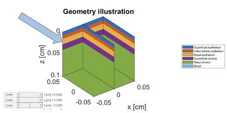
Prior research in biomedical optics has used a variety of 3D skin models, often simplifying tissue into broad categories such as air, epidermis, upper dermis, and lower dermis. However, for our investigation into oral tissue, we wanted to model a specialized, higher-resolution geometry for epithelial tissue rather than a standard skin model. This geometry divides the tissue into five distinct functional depths: superficial epithelium, intermediate epithelium, basal epithelium, superficial stroma, and deep stroma. | Prior research in biomedical optics has used a variety of 3D skin models, often simplifying tissue into broad categories such as air, epidermis, upper dermis, and lower dermis[[#References|[3]]]. However, for our investigation into oral tissue, we wanted to model a specialized, higher-resolution geometry for epithelial tissue rather than a standard skin model. This geometry divides the tissue into five distinct functional depths: superficial epithelium, intermediate epithelium, basal epithelium, superficial stroma, and deep stroma (see [[#Figure_4|Figure 4]]). | ||
This specific geometry is derived from Pavlova, the primary literature source guiding our modeling approach. While standard skin models often group cellular layers into a single "Epidermis," we wanted a more granular look into the layerings for detecting the subtle optical changes associated with oral precancer. Pavlova's work highlights that disease progression often starts in the lower epithelial layers, specifically the basal layer, before advancing upward. By separating the tissue into these fine-grained functional depths, our model is specifically designed to detect depth-dependent absorption changes caused by subsurface blood vessels. | This specific geometry is derived from Pavlova[[#References|[2]]], the primary literature source guiding our modeling approach. While standard skin models often group cellular layers into a single "Epidermis," we wanted a more granular look into the layerings for detecting the subtle optical changes associated with oral precancer. Pavlova's work highlights that disease progression often starts in the lower epithelial layers, specifically the basal layer, before advancing upward. By separating the tissue into these fine-grained functional depths, our model is specifically designed to detect depth-dependent absorption changes caused by subsurface blood vessels. | ||
<span id="Figure_4"></span> | |||
<div style="text-align:center;"> | <div style="text-align:center;"> | ||
[[File:5layermodel annotated.png|900px|center]] | [[File:5layermodel annotated.png|900px|center]] | ||
</div> | </div> | ||
<div style="text-align:center;">'''Figure | <div style="text-align:center;">'''Figure 4:''' Geometry illustration of the five-layer oral tissue model implemented in MCmatlab, differentiating between epithelial sublayers and stromal depths.</div> | ||
Functionally, the top three layers (Superficial, Intermediate, and Basal) represent the cellular epithelium. In Monte Carlo simulations, these layers are defined primarily by their scattering properties rather than absorption, reflecting the interaction of light with cellular structures. In contrast, the Superficial and Deep Stroma correspond to the underlying connective tissue, similar to the dermis in skin models. This is the critical region for our simulation, as it contains the blood vessels (the primary source of absorption) and collagen fibers (the primary source of fluorescence). To accurately simulate light transport within this complex structure in MCMatlab, unique optical coefficients (<math>\mu_a, \mu_s, g</math>) must be assigned to each of the five distinct regions shown in the geometry illustration. | Functionally, the top three layers (Superficial, Intermediate, and Basal) represent the cellular epithelium. In Monte Carlo simulations, these layers are defined primarily by their scattering properties rather than absorption, reflecting the interaction of light with cellular structures. In contrast, the Superficial and Deep Stroma correspond to the underlying connective tissue, similar to the dermis in skin models. This is the critical region for our simulation, as it contains the blood vessels (the primary source of absorption) and collagen fibers (the primary source of fluorescence). To accurately simulate light transport within this complex structure in MCMatlab, unique optical coefficients (<math>\mu_a, \mu_s, g</math>) must be assigned to each of the five distinct regions shown in the geometry illustration. | ||
| Line 145: | Line 152: | ||
In addition to the stratified epithelial layers, our simulation strategy evolved to address the spatial distribution of blood within the stroma. Initially, we considered modeling a single large blood vessel to represent blood spots. However, this approach proved unrealistic for capturing the optical effects of the diffuse microvasculature characteristic of the oral tissue. To address this limitation while maintaining a manageable simulation trade-off, we developed a "blood carpet" model. | In addition to the stratified epithelial layers, our simulation strategy evolved to address the spatial distribution of blood within the stroma. Initially, we considered modeling a single large blood vessel to represent blood spots. However, this approach proved unrealistic for capturing the optical effects of the diffuse microvasculature characteristic of the oral tissue. To address this limitation while maintaining a manageable simulation trade-off, we developed a "blood carpet" model. | ||
The blood carpet represents a continuous, dense layer of small blood vessels rather than a single discrete object. This configuration allows us to simulate the optical properties of a highly perfused vascular bed within the 3D geometry. This setup enables us to systematically vary the depth of the blood layer to determine how the "dark spot" signal changes as vessels are located deeper in the tissue. We generated several versions of the geometry where this blood carpet is positioned at specific depths ranging from the basal epithelium down to the deep stroma. | The blood carpet represents a continuous, dense layer of small blood vessels rather than a single discrete object. This configuration allows us to simulate the optical properties of a highly perfused vascular bed within the 3D geometry. This setup enables us to systematically vary the depth of the blood layer to determine how the "dark spot" signal changes as vessels are located deeper in the tissue. We generated several versions of the geometry where this blood carpet is positioned at specific depths ranging from the basal epithelium down to the deep stroma. [[#Figure_5|Figure 5]] below illustrates this progression, showing the blood carpet at depths of 200, 300, 400, 500, 600, and 800 μm. | ||
<span id="Figure_5"></span> | |||
<gallery mode="packed" heights="150px" > | <gallery mode="packed" heights="150px" > | ||
File:Bloodcarpet200arrow.png|Depth: 200 μm | File:Bloodcarpet200arrow.png|Depth: 200 μm | ||
| Line 155: | Line 163: | ||
File:Geometry_WithVessel_450nm_K1_depth800um.png|Depth: 800 μm | File:Geometry_WithVessel_450nm_K1_depth800um.png|Depth: 800 μm | ||
</gallery> | </gallery> | ||
<div style="text-align: center;">'''Figure | <div style="text-align: center;">'''Figure 5:''' Geometry simulations showing the 'blood carpet' at increasing depths within the tissue.</div> | ||
== Results == | == Results == | ||
| Line 167: | Line 175: | ||
<div style="text-align:center;">'''Fluence Distribution'''</div> | <div style="text-align:center;">'''Fluence Distribution'''</div> | ||
[[File:Fluence1.png|600px|center]] | [[File:Fluence1.png|600px|center]] | ||
<div style="text-align:center;">'''Figure | <div style="text-align:center;">'''Figure 6:''' Fluence comparison between keratinized and non-keratinized tissue</div> | ||
<p> | <p> | ||
Let us first examine the impact of keratin on the tissue by referring to Figure | Let us first examine the impact of keratin on the tissue by referring to Figure 5 (dashed lines represent non-keratinized tissue, solid lines represent keratinized tissue). Two main observations can be made. First, in keratinized tissue, there is a noticeable fluence peak in the superficial epithelium. This is explained by the higher scattering compared to absorption: for example, at 415 nm, the scattering coefficients are 170 (keratinized) versus 55 (non-keratinized), and at 450 nm, 140 versus 40. As a result, light is more likely to be scattered than absorbed, leading to higher fluence. Second, starting from the intermediate epithelium, the trend reverses: fluence becomes slightly higher in non-keratinized tissue. This can be interpreted as light being partially “trapped” in the superficial epithelium of keratinized tissue due to strong scattering, reducing the amount of light reaching deeper layers. | ||
</p> | </p> | ||
| Line 178: | Line 186: | ||
==== Measurable Results: Absorbance and Reflectance ==== | ==== Measurable Results: Absorbance and Reflectance ==== | ||
<span id="Figure_7"></span> | |||
<span id="Figure_8"></span> | |||
{| style="width:100%; text-align:center; border:none;" | {| style="width:100%; text-align:center; border:none;" | ||
| Line 190: | Line 199: | ||
|- | |- | ||
| '''Figure | | '''Figure 7:''' Absorbance comparison between keratinized and non-keratinized tissue | ||
| '''Figure | | '''Figure 8:''' Reflectance comparison between keratinized and non-keratinized tissue | ||
|} | |} | ||
| Line 202: | Line 211: | ||
</div> | </div> | ||
The results indicate that Absorbance is consistently higher at 415 nm compared to 450 nm, confirming the simulation correctly models the absorption peak of blood. Notably, Non-Keratinized (NK) tissue exhibits higher absorbance than Keratinized (K) tissue. This is due to the scattering properties of the keratin layer; in K tissue, photons are more likely to be scattered upward and exit the tissue before they can penetrate deep enough to be absorbed, resulting in a lower total absorbance value. | The results (see [[#Figure_7|Figure 7]]) indicate that Absorbance is consistently higher at 415 nm compared to 450 nm, confirming the simulation correctly models the absorption peak of blood. Notably, Non-Keratinized (NK) tissue exhibits higher absorbance than Keratinized (K) tissue. This is due to the scattering properties of the keratin layer; in K tissue, photons are more likely to be scattered upward and exit the tissue before they can penetrate deep enough to be absorbed, resulting in a lower total absorbance value. | ||
Reflectance is defined as the total photon energy exiting the tissue surface in the upward direction (measured at the surface), calculated as: | Reflectance is defined as the total photon energy exiting the tissue surface in the upward direction (measured at the surface), calculated as: | ||
| Line 210: | Line 219: | ||
</div> | </div> | ||
The reflectance data reveals distinct trends based on wavelength and tissue structure. Reflectance at 415 nm (Blue markers) is consistently lower than at 450 nm (Red markers) for both tissue types, as the strong blood absorption at 415 nm prevents photons from surviving the return trip to the detector. Furthermore, Keratinized tissue (K, Circles) demonstrates significantly higher reflectance than Non-Keratinized tissue (NK, Diamonds). This confirms that the keratin layer acts as a scattering "mirror" or shield: its high scattering coefficient redirects light back toward the surface before it reaches the deep stroma, effectively masking the signal from underlying blood vessels. | The reflectance data (see [[#Figure_8|Figure 8]]) reveals distinct trends based on wavelength and tissue structure. Reflectance at 415 nm (Blue markers) is consistently lower than at 450 nm (Red markers) for both tissue types, as the strong blood absorption at 415 nm prevents photons from surviving the return trip to the detector. Furthermore, Keratinized tissue (K, Circles) demonstrates significantly higher reflectance than Non-Keratinized tissue (NK, Diamonds). This confirms that the keratin layer acts as a scattering "mirror" or shield: its high scattering coefficient redirects light back toward the surface before it reaches the deep stroma, effectively masking the signal from underlying blood vessels. | ||
=== Influence of Blood Depth on the Optical Response === | === Influence of Blood Depth on the Optical Response === | ||
| Line 220: | Line 229: | ||
<p> | <p> | ||
Let us first consider the 415 nm results (Figure | Let us first consider the 415 nm results (Figure 8a–b). The most striking feature across all curves is the abrupt drop in fluence at the location of the blood layer (the “blood carpet”). This sharp decrease is a direct consequence of the high absorption of blood at 415 nm: many photon packets are absorbed in the blood layer, so the local fluence falls precipitously. This characteristic behavior—an abrupt fluence reduction at a specific depth—suggests a robust way to detect the presence of blood in the tissue: a marked dip in the measured fluence profile at the corresponding depth is a clear indicator of a highly absorbing blood layer (see Figure 8a and 8b). | ||
</p> | </p> | ||
| Line 228: | Line 237: | ||
<p> | <p> | ||
Comparing keratinized and non-keratinized tissues (Figure | Comparing keratinized and non-keratinized tissues (Figure 8a vs 8b and 8c vs 8d), both exhibit the same dramatic drop when the blood layer is reached. The principal difference is the small superficial bump in keratinized tissue: as discussed earlier, the high scattering in the keratinized superficial epithelium redirects and retains light near the surface, producing a local fluence enhancement (the bump) that is absent or much smaller in non-keratinized tissue. | ||
</p> | </p> | ||
<p> | <p> | ||
The same sequence of features appears at 450 nm (Figure | The same sequence of features appears at 450 nm (Figure 8c–d), but overall fluence values are higher than at 415 nm. This is expected because absorption coefficients are lower at 450 nm, so fewer photons are lost to absorption and more light penetrates deeper. Consequently, the fluence drop at the blood layer is less pronounced at 450 nm than at 415 nm: 415 nm lies closer to a blood absorption peak and is therefore more sensitive to the presence of blood, while 450 nm is comparatively less absorbed and shows a milder dip. | ||
</p> | </p> | ||
<p> | <p> | ||
In summary, the combination of (i) a sharp fluence decrease at the blood depth, (ii) a small post-drop increase driven by longer photon path lengths in the less-absorbing tissue, and (iii) the superficial bump in keratinized tissue (due to strong scattering) provides a consistent, physically intuitive picture across wavelengths and tissue types (see Figure | In summary, the combination of (i) a sharp fluence decrease at the blood depth, (ii) a small post-drop increase driven by longer photon path lengths in the less-absorbing tissue, and (iii) the superficial bump in keratinized tissue (due to strong scattering) provides a consistent, physically intuitive picture across wavelengths and tissue types (see Figure 8a–d). | ||
</p> | </p> | ||
| Line 253: | Line 262: | ||
| (d) Fluence at 450 nm<br/>Keratinized tissue | | (d) Fluence at 450 nm<br/>Keratinized tissue | ||
|- | |- | ||
| colspan="2" style="text-align:center;" | '''Figure | | colspan="2" style="text-align:center;" | '''Figure 9:''' Fluence distribution as a function of depth for different wavelengths and tissue types | ||
|} | |} | ||
==== Measurable Results: Absorbance and Reflectance ==== | ==== Measurable Results: Absorbance and Reflectance ==== | ||
<span id="Figure_10"></span> | |||
<span id="Figure_11"></span> | |||
{| style="width:100%; text-align:center; border:none;" | {| style="width:100%; text-align:center; border:none;" | ||
|- | |- | ||
| Line 264: | Line 275: | ||
[[File:Absorbance_vs_depth_4curves.png|450px]] | [[File:Absorbance_vs_depth_4curves.png|450px]] | ||
<div>'''Figure | <div>'''Figure 10:''' Absorbance as a function of blood depth for different wavelengths and tissue types</div> | ||
</div> | </div> | ||
| <div> | | <div> | ||
| Line 271: | Line 282: | ||
[[File:Reflectance_vs_depth_4curves.png|450px]] | [[File:Reflectance_vs_depth_4curves.png|450px]] | ||
<div>'''Figure | <div>'''Figure 11:''' Reflectance as a function of blood depth for different wavelengths and tissue types</div> | ||
</div> | </div> | ||
|} | |} | ||
| Line 277: | Line 288: | ||
To quantify the impact of vascular depth on the optical signal, we analyzed the total absorbance and reflectance as a function of the blood carpet's position (varying from 200 μm to 800 μm). | To quantify the impact of vascular depth on the optical signal, we analyzed the total absorbance and reflectance as a function of the blood carpet's position (varying from 200 μm to 800 μm). | ||
Absorbance is defined here as the total amount of light energy lost (absorbed) inside the tissue volume. The graph above displays Absorbance vs. Vessel Depth, illustrating a trend similar to exponential decay. As the blood vessel is positioned deeper within the tissue, the total absorbance decreases. This occurs because the excitation light is attenuated by the overlying tissue layers before it reaches the blood; fewer photons reach the deep vessels, resulting in less energy absorption. The curve decays until it asymptotes to a final "control value," representing the baseline absorbance of bloodless tissue. The rate of this decay changes noticeably depending on whether the vessel is located in the epithelium or the stroma, reflecting the different attenuation properties of these tissue layers. Absorbance is consistently higher for 415 nm wavelength compared to 450 nm, confirming the higher sensitivity of the 415 nm wavelength to hemoglobin. Absorbance is higher in Non-Keratinized (NK) tissue than in Keratinized (K) tissue. In K-tissue, the highly scattering superficial layer reflects a significant portion of photons back out of the tissue before they can penetrate deep enough to be absorbed by the blood, effectively "shielding" the signal. | Absorbance is defined here as the total amount of light energy lost (absorbed) inside the tissue volume. The graph above (see [[#Figure_10|Figure 10]]) displays Absorbance vs. Vessel Depth, illustrating a trend similar to exponential decay. As the blood vessel is positioned deeper within the tissue, the total absorbance decreases. This occurs because the excitation light is attenuated by the overlying tissue layers before it reaches the blood; fewer photons reach the deep vessels, resulting in less energy absorption. The curve decays until it asymptotes to a final "control value," representing the baseline absorbance of bloodless tissue. The rate of this decay changes noticeably depending on whether the vessel is located in the epithelium or the stroma, reflecting the different attenuation properties of these tissue layers. Absorbance is consistently higher for 415 nm wavelength compared to 450 nm, confirming the higher sensitivity of the 415 nm wavelength to hemoglobin. Absorbance is higher in Non-Keratinized (NK) tissue than in Keratinized (K) tissue. In K-tissue, the highly scattering superficial layer reflects a significant portion of photons back out of the tissue before they can penetrate deep enough to be absorbed by the blood, effectively "shielding" the signal. | ||
Reflectance is defined as the total photon energy exiting the tissue surface upward (i.e., the light that comes back out to the detector). It is measured at the surface. The graph demonstrates that Reflectance is consistently higher in Keratinized (K) tissue compared to Non-Keratinized (NK) tissue. This is driven by the high scattering coefficient (<math>\mu_s</math>) of the keratin layer, which acts like a diffusive mirror, redirecting photons back toward the surface. Reflectance generally follows an inverse trend to absorbance; where absorbance is high (e.g., shallow vessels in NK tissue), reflectance is low because the energy is trapped. As the vessel moves deeper and absorbs less light, the total reflectance recovers toward the baseline value. | Reflectance is defined as the total photon energy exiting the tissue surface upward (i.e., the light that comes back out to the detector). It is measured at the surface. The graph (see [[#Figure_11|Figure 11]]) demonstrates that Reflectance is consistently higher in Keratinized (K) tissue compared to Non-Keratinized (NK) tissue. This is driven by the high scattering coefficient (<math>\mu_s</math>) of the keratin layer, which acts like a diffusive mirror, redirecting photons back toward the surface. Reflectance generally follows an inverse trend to absorbance; where absorbance is high (e.g., shallow vessels in NK tissue), reflectance is low because the energy is trapped. As the vessel moves deeper and absorbs less light, the total reflectance recovers toward the baseline value. | ||
== Discussion and Conclusions == | == Discussion and Conclusions == | ||
| Line 286: | Line 297: | ||
To address these constraints, future research must expand beyond purely computational modeling to include physical validation. Specifically, acquiring physical measurements of reflectance across a broader spectral range is essential to establish a ground-truth benchmark for these coefficients. Validating the MCmatlab results against in-vivo measurements would allow for precise calibration of the simulation parameters, bridging the gap between theoretical assumptions and biological reality for such a critical health diagnosis. | To address these constraints, future research must expand beyond purely computational modeling to include physical validation. Specifically, acquiring physical measurements of reflectance across a broader spectral range is essential to establish a ground-truth benchmark for these coefficients. Validating the MCmatlab results against in-vivo measurements would allow for precise calibration of the simulation parameters, bridging the gap between theoretical assumptions and biological reality for such a critical health diagnosis. | ||
An important takeaway from our study concerns the difference between theoretical and experimentally measurable quantities. While our fluence-depth plots clearly reveal the presence of blood vessels—demonstrating a distinct local drop in fluence at the vessel depth—fluence itself is not a quantity that can be measured in practice. It is a purely theoretical output of the Monte Carlo model. In contrast, absorbance represents the measurable optical signal in real experiments. However, our results show that for both wavelengths (415 nm and 450 nm), the absorbance returned to values nearly identical to the control simulations, even when a vessel was placed as deep as 900 μm. This was unexpected, since 450 nm was anticipated to penetrate deeper than 415 nm and therefore to display a greater sensitivity to subsurface vessels. The fact that no measurable difference appears between control and vessel-inclusion cases suggests that, under our current model assumptions, the presence of deep blood vessels may not produce a detectable absorbance change — or alternatively, that the model requires refinement to better capture depth-dependent absorption effects. | |||
== References == | == References == | ||
| Line 304: | Line 317: | ||
<li>Morgan, D. (2024). How does the VELscope work? ''VELscope''. [https://velscope.com/how-does-the-velscope-work/ Link]</li> | <li>Morgan, D. (2024). How does the VELscope work? ''VELscope''. [https://velscope.com/how-does-the-velscope-work/ Link]</li> | ||
<li>Johnson, E. (2025). VELscope Oral Cancer Detection Device. [https://www.drericjohnson.com/san-clemente-ca/velscope-oral-cancer-detection-device/ Link]</li> | |||
</ol> | </ol> | ||
== Appendix == | == Appendix I == | ||
Our code can be found at https://github.com/Lisy13012/Simulation-of-Optical-Response-in-Oral-Tissue. | Our code can be found at https://github.com/Lisy13012/Simulation-of-Optical-Response-in-Oral-Tissue. | ||
== Appendix II == | |||
Lise worked on the coefficient plot generations using MC simulations, literature review, and focused on fluence interpretations. | |||
Sylvia worked on geometry and absorbance/reflectance interpretations, literature review, and understanding MCMatlab. | |||
Latest revision as of 18:40, 11 December 2025
Introduction
Oral cancer remains a significant global health challenge, where early detection is the most critical factor in improving survival rates. Traditionally, screening has relied on standard white light examinations; however, this method is limited by the human eye's error-prone ability to detect subtle lesions that may not clearly manifest under typical examinations. To address these limitations, the VELscope[8] has emerged as a promising, non-invasive, and rapid technology for efficiently screening oral tissue.

Leading this technological shift is the VELscope, a handheld device that utilizes blue excitation light to visualize tissue abnormalities. Under VELscope illumination, healthy tissue emits a pale green fluorescence due to fluorophores such as collagen, whereas cancerous tissue typically appears as a distinct "dark spot" due to a loss of fluorescence[8]. This contrast enhancement addresses the limitations of incandescent white light, clearly illuminating potential lesions that might otherwise go unnoticed.
Despite the clinical utility of the VELscope, a significant gap remains in the interpretation of these "dark spots." While the device is effective at identifying areas of low fluorescence, it lacks specificity regarding the biological cause of the signal loss; it could simply be a concentrated blood spot. Crucially, limited research has been conducted to distinguish between dark spots caused by cancer, and those caused by benign "blood spots" resulting from trauma, infection, or inflammation. Hemoglobin is a potent absorber of light in the blue-green spectrum, and therefore increased blood volume can mimic the optical appearance of a cancerous lesion by absorbing the fluorescence before it reaches the detector. This ambiguity presents a diagnostic challenge: a "dark spot" could represent a malignant breakdown of collagen, or it could simply represent a localized accumulation of blood due to another health issue. To improve the specificity of autofluorescence screening, it is essential to decouple the optical effects of blood absorption from true tissue fluorescence.
In this paper, we address this challenge by simulating the optical response of oral tissue using Monte Carlo modeling in MCmatlab. Prior research, notably by Pavlova et al.[2], has successfully employed multi-layered Monte Carlo models to predict fluorescence spectra in oral neoplasia, establishing the importance of site-specific optical properties and layered tissue geometries. However, they primarily focused on intrinsic fluorophores rather than the specific depth-dependent reflectance signatures caused by variable blood accumulation. By computationally modeling the interaction of light with varying depths of blood vessels and tissue layers -- specifically comparing the response at the highly absorbing 415 nm wavelength versus the more penetrating 450 nm wavelength -- we aim to investigate the impact of blood on tissue reflectance. This study seeks to provide a new theoretical framework for detecting benign blood absorption in oral tissue, potentially reducing false positives in optical oral cancer screening.
Background
Previous Work
The main objective of this work is to investigate how the presence of blood at different depths within oral tissue influences the optical response when illuminated at two wavelengths: 415 nm, corresponding to the peak of blood absorption, and 450 nm. Our analysis focuses particularly on three key simulated quantities: fluence, absorption and reflectance.
A substantial body of literature has examined how tissue morphology, biochemical composition, and structural organization affect optical signals in the oral cavity. Several studies have used Monte Carlo simulations to characterize light transport in multilayered epithelial tissues and to understand how scattering, absorption, and fluorescence vary between healthy and pathological sites. For example, VELscope-based diagnostic approaches rely on differences in autofluorescence between normal and diseased mucosa, as discussed in Vibhute et al. [1], and in manufacturer technical notes such as Morgan [8]. These studies highlight the importance of accurately modeling tissue-layer optical properties to interpret measured signals.
Among simulation-based approaches, the work of Pavlova et al. [2] is particularly relevant: their study aims to predict fluorescence spectra from normal, inflammatory, and neoplastic oral sites using Monte Carlo modeling with site-specific optical parameters. Their results demonstrate that changes in epithelial thickness, scattering coefficients, and subepithelial absorption—especially due to blood—significantly influence the detected fluorescence signal.
Our approach builds directly on the methodology of Pavlova et al., adopting and adapting their five-layer oral tissue model for our own simulations. All photon transport computations were performed using MCmatlab [5], a voxel-based Monte Carlo simulation framework. Optical properties of blood were taken from the extensive review by Jacques [4], while tissue optical parameters around 415 nm were extracted from Pavlova’s dataset.
Other relevant modeling efforts in the literature include radiative transfer analyses applied to biological tissues (ScienceDirect Topics overview [6]) and investigations of optical properties in normal versus pathological skin by Salomatina et al. [7], which reinforce the importance of correctly representing absorption and scattering contrasts between layers. Additionally, blood oxygen modeling studies—such as Sharma et al. [3]—illustrate how hemoglobin absorption spectra influence reflectance measurements, supporting the need to analyze the specific contribution of subsurface blood layers.
Optical Tissue Properties in the Literature
| Tissue Layer | μa [cm⁻¹] 415 nm | μs [cm⁻¹] 415 nm | μa [cm⁻¹] 450 nm | μs [cm⁻¹] 450 nm |
|---|---|---|---|---|
| Superficial epithelium | 3.0 | 170 (keratinized) / 55 (non keratinized) | 2.1 | 140 (keratinized) / 40 (non keratinized) |
| Intermediate epithelium | 3.0 | 55 | 2.1 | 40 |
| Basal epithelium | 3.0 | 55 | 2.1 | 40 |
| Superficial stroma | 6.22 | 267 | 3.11 | 248.5 |
| Deep stroma | 6.22 | 267 | 3.11 | 248.5 |
| Blood | 262 | 37.8 | 30 | 31.1 |
The optical behavior of oral tissue has been widely investigated, particularly through the study of its absorption and scattering characteristics across different anatomical layers. In our work, we distinguish between keratinized and non-keratinized epithelium, since keratin is present in tongue tissue but absent in buccal mucosa — a distinction known to substantially modify scattering properties due to microstructural differences in the superficial epithelial layer.
All optical coefficients at 415 nm were taken directly from Pavlova et al.'s Monte Carlo study of oral fluorescence, which provides wavelength-specific absorption and scattering parameters for a five-layer oral tissue model[2]. For 450 nm, scattering coefficients were computed following the same methodology as Pavlova, using a power-law spectral dependence commonly applied to biological tissues[4].
However, because realistic absorption values at 450 nm were needed, we adopted a spectral-ratio approach based on experimental optical measurements from Salomatina et al. (2006), who quantified absorption and scattering in human epidermis and dermis across the visible spectrum7. Since hemoglobin is the dominant absorber in this spectral range, the ratio between 415 nm and 450 nm absorption in skin tissue largely reflects variations in blood content. By applying these experimentally measured ratios to the 415 nm absorption values from Pavlova, we derived physically consistent absorption coefficients at 450 nm adapted to oral tissue.
Overall, this parameter-construction method ensures that the simulated optical response captures both oral-tissue–specific morphology (via Pavlova's model) and realistic wavelength-dependent absorption behavior (via Salomatina's spectral data), providing a more faithful representation of how blood and tissue layers interact with blue-visible illumination.
Methods
Monte Carlo Simulation Principle
A simple Monte Carlo simulation can be used to estimate the value of π by comparing areas of a circle and a square. First, the geometric domain is defined, consisting of a square whose side is equal to twice the radius of the circle, so that the circle is fully inscribed within the square (see Figure 2a). A large number of points are then generated randomly and uniformly within the square. Each point is classified according to whether it lies inside the circle or outside, and the number of points falling within the circle is counted (see Figure 2b). The ratio of the number of points inside the circle to the total number of points in the square approaches the ratio of the areas of the circle and the square: . Multiplying this ratio by four therefore provides an estimate of π. This example illustrates how probabilistic sampling can be used to approximate geometric quantities.
The name “Monte Carlo” comes from the famous casinos in Monte Carlo, reflecting the stochastic (random) nature of the method. Monte Carlo simulations rely on the law of large numbers, meaning that in order to obtain accurate results, it is crucial to generate a sufficiently large number of random points so that the results converge to an asymptotic value.

|

|
| (a) Definition of the geometric domain | (b) Random point generation, classification, and counting |
| Figure 2: Basic Monte Carlo simulation to compute π | |
Monte Carlo Simulation for Light Propagation
Monte Carlo simulations can be applied to model the propagation of light in scattering and absorbing media, such as biological tissue. First, the geometric domain is defined, specifying the optical properties of the medium and the spatial grid where energy deposition will be recorded. A photon packet is then launched from the source with an initial weight (see Figure 3a). The photon propagates in a straight line over a free path. The probability of an interaction occurring in the infinitesimal path interval is , where (see Figure 3b). Note that the free path follows an exponential distribution.
Upon reaching an interaction, the photon can be absorbed or scattered according to probabilities and . If scattering occurs, the anisotropy factor determines the preferential direction: corresponds to forward scattering, and larger values imply scattering at smaller angles, meaning the photon is deflected less from its initial direction. Here, , so scattering occurs mostly in the forward direction with small angles (see Figure 3c). During absorption events, the absorbed energy is , and the photon weight is updated to , with the remaining weight continuing to propagate (see Figure 3d).
By repeating these steps for many photon packets, the simulation statistically reconstructs macroscopic quantities such as fluence, reflectance, and transmittance in the medium.

|

|

|

|
| (a) Launching a photon packet | (b) Straight-line propagation over a free path | (c) Interaction event | (d) Updating the Photon Weight |
| Figure 3: Monte Carlo simulation for light | |||
MC Matlab
To simulate the optical response of oral tissue, we utilized MCMatlab, an open-source, MATLAB-based software package designed to model light transport in complex, scattering media such as biological tissue[5]. This platform is particularly valuable for its ability to handle 3D geometries and diverse light source configurations, allowing for the simulation of intricate physiological structures. The fundamental mathematical model governing MCMatlab is the Radiative Transfer Equation (RTE)[6]. The RTE describes the conservation of energy as light propagates through a medium, accounting for energy loss via absorption and scattering, as well as energy gain from scattering events into the direction of propagation. It tracks the radiance flowing through a volumetric medium as a function of position, direction, and wavelength. Due to the complexity of solving the RTE analytically in biological tissues, MCMatlab employs Monte Carlo simulations to solve it stochastically.
The Monte Carlo method models light transport by tracking the so-called "random walks"[5] of millions of individual photons. This stochastic approach is a core assumption necessary for the software to function; the motion of each photon is sampled randomly based on the optical properties of the medium. Notably, the distance a photon travels before interacting with the tissue (the step size) is determined by the medium's attenuation coefficient. For example, if the tissue has high attenuation at a specific wavelength, the step sizes are statistically shorter, leading to shallower penetration depths. At every interaction point, the photon may be absorbed, losing "weight", or scattered into a new direction.
A critical feature of MCMatlab is its ability to characterize tissue using four primary optical parameters, which allow users to accurately model how light interacts with different tissue components. For this study, we focused on the following parameters, consistent with existing literature on oral tissue modeling:
- Absorption Coefficient (): Defines the probability of photon absorption per unit path length.
- Scattering Coefficient (): Describes the probability of photon scattering per unit path length.
- Anisotropy (): Represents the directionality of scattering.
- Refractive Index (): The ratio of the velocity of light in a vacuum to its velocity in the specified medium.
It is important to note that the physics engine behind MCMatlab is not inherently wavelength-specific; rather, the simulation is entirely controlled by these input coefficients. By adjusting these coefficients to match empirical data for specific wavelengths (e.g., 415 nm vs. 450 nm), we were able to simulate our desired physiological conditions.
Five Layer Model and Geometry
Prior research in biomedical optics has used a variety of 3D skin models, often simplifying tissue into broad categories such as air, epidermis, upper dermis, and lower dermis[3]. However, for our investigation into oral tissue, we wanted to model a specialized, higher-resolution geometry for epithelial tissue rather than a standard skin model. This geometry divides the tissue into five distinct functional depths: superficial epithelium, intermediate epithelium, basal epithelium, superficial stroma, and deep stroma (see Figure 4).
This specific geometry is derived from Pavlova[2], the primary literature source guiding our modeling approach. While standard skin models often group cellular layers into a single "Epidermis," we wanted a more granular look into the layerings for detecting the subtle optical changes associated with oral precancer. Pavlova's work highlights that disease progression often starts in the lower epithelial layers, specifically the basal layer, before advancing upward. By separating the tissue into these fine-grained functional depths, our model is specifically designed to detect depth-dependent absorption changes caused by subsurface blood vessels.

Functionally, the top three layers (Superficial, Intermediate, and Basal) represent the cellular epithelium. In Monte Carlo simulations, these layers are defined primarily by their scattering properties rather than absorption, reflecting the interaction of light with cellular structures. In contrast, the Superficial and Deep Stroma correspond to the underlying connective tissue, similar to the dermis in skin models. This is the critical region for our simulation, as it contains the blood vessels (the primary source of absorption) and collagen fibers (the primary source of fluorescence). To accurately simulate light transport within this complex structure in MCMatlab, unique optical coefficients () must be assigned to each of the five distinct regions shown in the geometry illustration.
In addition to the stratified epithelial layers, our simulation strategy evolved to address the spatial distribution of blood within the stroma. Initially, we considered modeling a single large blood vessel to represent blood spots. However, this approach proved unrealistic for capturing the optical effects of the diffuse microvasculature characteristic of the oral tissue. To address this limitation while maintaining a manageable simulation trade-off, we developed a "blood carpet" model.
The blood carpet represents a continuous, dense layer of small blood vessels rather than a single discrete object. This configuration allows us to simulate the optical properties of a highly perfused vascular bed within the 3D geometry. This setup enables us to systematically vary the depth of the blood layer to determine how the "dark spot" signal changes as vessels are located deeper in the tissue. We generated several versions of the geometry where this blood carpet is positioned at specific depths ranging from the basal epithelium down to the deep stroma. Figure 5 below illustrates this progression, showing the blood carpet at depths of 200, 300, 400, 500, 600, and 800 μm.
-
 Depth: 200 μm
 -
 Depth: 300 μm
 -
 Depth: 400 μm
 -
 Depth: 500 μm
 -
 Depth: 600 μm
 -
 Depth: 800 μm


Results
Influence of Keratin on the Optical Response
Theoretical Results: Fluence
All graphs are presented in arbitrary units because the Monte Carlo simulations rely on photon weights W, which do not represent the exact number of photons. Fluence is calculated as , where wi is the weight of photon packet i, μa is the absorption coefficient of the medium traversed, and is the straight-line path length of the photon packet. In practice, fluence can be interpreted as the energy density within the tissue, or more intuitively, as a measure of how much light is present at a given depth z.

Let us first examine the impact of keratin on the tissue by referring to Figure 5 (dashed lines represent non-keratinized tissue, solid lines represent keratinized tissue). Two main observations can be made. First, in keratinized tissue, there is a noticeable fluence peak in the superficial epithelium. This is explained by the higher scattering compared to absorption: for example, at 415 nm, the scattering coefficients are 170 (keratinized) versus 55 (non-keratinized), and at 450 nm, 140 versus 40. As a result, light is more likely to be scattered than absorbed, leading to higher fluence. Second, starting from the intermediate epithelium, the trend reverses: fluence becomes slightly higher in non-keratinized tissue. This can be interpreted as light being partially “trapped” in the superficial epithelium of keratinized tissue due to strong scattering, reducing the amount of light reaching deeper layers.
Next, the influence of wavelength is considered. Comparing 415 nm and 450 nm, fluence is higher at 450 nm, which is consistent with lower absorption coefficients at this wavelength. Finally, a prominent feature appears between the epithelium and the stroma for all four curves: a large fluence increase. This arises because the absorption coefficient is effectively doubled in that region, which, according to the formula above, temporarily increases fluence. Beyond this peak, all curves gradually decrease with depth due to absorption.
Measurable Results: Absorbance and Reflectance
| Absorbance Distribution | Reflectance Distribution |
|---|---|

|

|
| Figure 7: Absorbance comparison between keratinized and non-keratinized tissue | Figure 8: Reflectance comparison between keratinized and non-keratinized tissue |
To quantify the optical interactions within the tissue, we analyzed two complementary metrics: Absorbance and Reflectance. Absorbance is defined as the fraction of photon energy lost inside the tissue. It is calculated by summing the weight loss of all photon packets during simulation:

The results (see Figure 7) indicate that Absorbance is consistently higher at 415 nm compared to 450 nm, confirming the simulation correctly models the absorption peak of blood. Notably, Non-Keratinized (NK) tissue exhibits higher absorbance than Keratinized (K) tissue. This is due to the scattering properties of the keratin layer; in K tissue, photons are more likely to be scattered upward and exit the tissue before they can penetrate deep enough to be absorbed, resulting in a lower total absorbance value.
Reflectance is defined as the total photon energy exiting the tissue surface in the upward direction (measured at the surface), calculated as:

The reflectance data (see Figure 8) reveals distinct trends based on wavelength and tissue structure. Reflectance at 415 nm (Blue markers) is consistently lower than at 450 nm (Red markers) for both tissue types, as the strong blood absorption at 415 nm prevents photons from surviving the return trip to the detector. Furthermore, Keratinized tissue (K, Circles) demonstrates significantly higher reflectance than Non-Keratinized tissue (NK, Diamonds). This confirms that the keratin layer acts as a scattering "mirror" or shield: its high scattering coefficient redirects light back toward the surface before it reaches the deep stroma, effectively masking the signal from underlying blood vessels.
Influence of Blood Depth on the Optical Response
Theoretical Results: Fluence
As a quick reminder, fluence is computed as , where wi is the weight of photon packet i, μa is the absorption coefficient of the medium traversed, and is the straight-line path length travelled by that photon packet. In practice, fluence represents the energy density within the tissue: intuitively, it measures how much light is present at a given depth z.
Let us first consider the 415 nm results (Figure 8a–b). The most striking feature across all curves is the abrupt drop in fluence at the location of the blood layer (the “blood carpet”). This sharp decrease is a direct consequence of the high absorption of blood at 415 nm: many photon packets are absorbed in the blood layer, so the local fluence falls precipitously. This characteristic behavior—an abrupt fluence reduction at a specific depth—suggests a robust way to detect the presence of blood in the tissue: a marked dip in the measured fluence profile at the corresponding depth is a clear indicator of a highly absorbing blood layer (see Figure 8a and 8b).
Immediately after the drop, the fluence shows a modest recovery (a small bump). This can be explained using the fluence formula: photon weights wi can only decrease with depth (we do not generate photons), so the only way for to increase locally is for the path lengths in the subsequent medium to increase. In other words, photons that survive the blood layer tend to travel longer straight-line distances in the less-absorbing tissue below, increasing the contribution of to the fluence and producing the observed small rise.
Comparing keratinized and non-keratinized tissues (Figure 8a vs 8b and 8c vs 8d), both exhibit the same dramatic drop when the blood layer is reached. The principal difference is the small superficial bump in keratinized tissue: as discussed earlier, the high scattering in the keratinized superficial epithelium redirects and retains light near the surface, producing a local fluence enhancement (the bump) that is absent or much smaller in non-keratinized tissue.
The same sequence of features appears at 450 nm (Figure 8c–d), but overall fluence values are higher than at 415 nm. This is expected because absorption coefficients are lower at 450 nm, so fewer photons are lost to absorption and more light penetrates deeper. Consequently, the fluence drop at the blood layer is less pronounced at 450 nm than at 415 nm: 415 nm lies closer to a blood absorption peak and is therefore more sensitive to the presence of blood, while 450 nm is comparatively less absorbed and shows a milder dip.
In summary, the combination of (i) a sharp fluence decrease at the blood depth, (ii) a small post-drop increase driven by longer photon path lengths in the less-absorbing tissue, and (iii) the superficial bump in keratinized tissue (due to strong scattering) provides a consistent, physically intuitive picture across wavelengths and tissue types (see Figure 8a–d).

|

|
| (a) Fluence at 415 nm Non-keratinized tissue |
(b) Fluence at 415 nm Keratinized tissue |

|

|
| (c) Fluence at 450 nm Non-keratinized tissue |
(d) Fluence at 450 nm Keratinized tissue |
| Figure 9: Fluence distribution as a function of depth for different wavelengths and tissue types | |
Measurable Results: Absorbance and Reflectance
Absorbance Distribution
Figure 10: Absorbance as a function of blood depth for different wavelengths and tissue types
|
Reflectance Distribution
Figure 11: Reflectance as a function of blood depth for different wavelengths and tissue types
|


To quantify the impact of vascular depth on the optical signal, we analyzed the total absorbance and reflectance as a function of the blood carpet's position (varying from 200 μm to 800 μm).
Absorbance is defined here as the total amount of light energy lost (absorbed) inside the tissue volume. The graph above (see Figure 10) displays Absorbance vs. Vessel Depth, illustrating a trend similar to exponential decay. As the blood vessel is positioned deeper within the tissue, the total absorbance decreases. This occurs because the excitation light is attenuated by the overlying tissue layers before it reaches the blood; fewer photons reach the deep vessels, resulting in less energy absorption. The curve decays until it asymptotes to a final "control value," representing the baseline absorbance of bloodless tissue. The rate of this decay changes noticeably depending on whether the vessel is located in the epithelium or the stroma, reflecting the different attenuation properties of these tissue layers. Absorbance is consistently higher for 415 nm wavelength compared to 450 nm, confirming the higher sensitivity of the 415 nm wavelength to hemoglobin. Absorbance is higher in Non-Keratinized (NK) tissue than in Keratinized (K) tissue. In K-tissue, the highly scattering superficial layer reflects a significant portion of photons back out of the tissue before they can penetrate deep enough to be absorbed by the blood, effectively "shielding" the signal.
Reflectance is defined as the total photon energy exiting the tissue surface upward (i.e., the light that comes back out to the detector). It is measured at the surface. The graph (see Figure 11) demonstrates that Reflectance is consistently higher in Keratinized (K) tissue compared to Non-Keratinized (NK) tissue. This is driven by the high scattering coefficient () of the keratin layer, which acts like a diffusive mirror, redirecting photons back toward the surface. Reflectance generally follows an inverse trend to absorbance; where absorbance is high (e.g., shallow vessels in NK tissue), reflectance is low because the energy is trapped. As the vessel moves deeper and absorbs less light, the total reflectance recovers toward the baseline value.
Discussion and Conclusions
A primary limitation of this study is the scarcity of consistent experimental data in the literature regarding optical properties, specifically absorption and scattering coefficients—within the narrow 415 nm and 450 nm spectral bands. This necessitated a reliance on theoretical approximations rather than empirical values to parameterize the model. Furthermore, the study relies exclusively on computational predictions via MCmatlab, which inherently simplifies the physical physics of light transport. The simulation treats light as discrete photon packets governing by stochastic random walks, thereby neglecting wave phenomena, and assumes that optical properties are uniform and constant within each defined voxel. Consequently, the idealized 5-layer geometry may oversimplify complex biological factors, such as variable vessel depth.
To address these constraints, future research must expand beyond purely computational modeling to include physical validation. Specifically, acquiring physical measurements of reflectance across a broader spectral range is essential to establish a ground-truth benchmark for these coefficients. Validating the MCmatlab results against in-vivo measurements would allow for precise calibration of the simulation parameters, bridging the gap between theoretical assumptions and biological reality for such a critical health diagnosis.
An important takeaway from our study concerns the difference between theoretical and experimentally measurable quantities. While our fluence-depth plots clearly reveal the presence of blood vessels—demonstrating a distinct local drop in fluence at the vessel depth—fluence itself is not a quantity that can be measured in practice. It is a purely theoretical output of the Monte Carlo model. In contrast, absorbance represents the measurable optical signal in real experiments. However, our results show that for both wavelengths (415 nm and 450 nm), the absorbance returned to values nearly identical to the control simulations, even when a vessel was placed as deep as 900 μm. This was unexpected, since 450 nm was anticipated to penetrate deeper than 415 nm and therefore to display a greater sensitivity to subsurface vessels. The fact that no measurable difference appears between control and vessel-inclusion cases suggests that, under our current model assumptions, the presence of deep blood vessels may not produce a detectable absorbance change — or alternatively, that the model requires refinement to better capture depth-dependent absorption effects.
References
- Vibhute, N. A., Jagtap, S. V., & Patil, S. V. (2021). Velscope guided oral cancer screening: A ray of hope in early oral cancer diagnosis. Journal of Oral and Maxillofacial Pathology, 25(3), 548–549. DOI
- Pavlova, I. Fluorescence spectroscopy of oral tissue: Monte Carlo modeling with site-specific tissue properties.
- Sharma, R., Joshi, P., & Deopujari, A. Blood oxygen modelling from skin reflectance. Project report.
- Jacques, S. L. (2013). Optical properties of biological tissues: A review. Physics in Medicine & Biology, 58(11), R37–R61.
- MathWorks. (2023). MCmatlab: A Monte Carlo simulation for photon transport in 3D voxel space. Link
- Radiative Transfer Equation. ScienceDirect Topics. Link
- Salomatina, E. et al. (2006). Optical properties of normal and cancerous human skin in the visible and near-infrared spectral range. Journal of Biomedical Optics, 11(6), 064026.
- Morgan, D. (2024). How does the VELscope work? VELscope. Link
- Johnson, E. (2025). VELscope Oral Cancer Detection Device. Link
Appendix I
Our code can be found at https://github.com/Lisy13012/Simulation-of-Optical-Response-in-Oral-Tissue.
Appendix II
Lise worked on the coefficient plot generations using MC simulations, literature review, and focused on fluence interpretations. Sylvia worked on geometry and absorbance/reflectance interpretations, literature review, and understanding MCMatlab.