Joelle Dowling: Difference between revisions
imported>Student221 |
imported>Student221 |
||
| (15 intermediate revisions by the same user not shown) | |||
| Line 36: | Line 36: | ||
Since this project creates and tests the model, we have "training" datasets and test datasets. The former are referred to as Measurements1 and the latter, Measurements2. Measurements1 contains radiance data and DNG files for the MCC illuminated by one of three illuminants, Tungsten (A), Cool White Fluorescent (CWF), and Daylight (DAY). Measurements2 contains radiance data and DNG files for the MCC illuminated by a Tungsten light. All the camera images are taken with the same ISO Speed, but have different Exposure Times. | Since this project creates and tests the model, we have "training" datasets and test datasets. The former are referred to as Measurements1 and the latter, Measurements2. Measurements1 contains radiance data and DNG files for the MCC illuminated by one of three illuminants, Tungsten (A), Cool White Fluorescent (CWF), and Daylight (DAY). Measurements2 contains radiance data and DNG files for the MCC illuminated by a Tungsten light. All the camera images are taken with the same ISO Speed, but have different Exposure Times. | ||
We have to extract the RGB values from the DNG files. For this, we use ISETCAM's sensor functions. First we read the DNG file using <code>sensorDNGRead</code>. Then we open a window that displays the sensor image using, <code>sensorWindow</code>.From there we estimate rectangles where the 24 boxes are on the MCC using the <code>chartCornerpoints</code> function. An example of the sensor window with the rectangles charted is shown in Figure 2. If we are satisfied by the placement of the rectangles, we get the digital values from each square using the function <code>chartRectsData</code> | We have to extract the RGB values from the DNG files. For this, we use ISETCAM's sensor functions. First we read the DNG file using <code>sensorDNGRead</code>. Then we open a window that displays the sensor image using, <code>sensorWindow</code>.From there we estimate rectangles where the 24 boxes are on the MCC using the <code>chartCornerpoints</code> function. An example of the sensor window with the rectangles charted is shown in Figure 2. If we are satisfied by the placement of the rectangles, we get the digital values from each square using the function <code>chartRectsData</code>. We then get the mean and standard deviation of the RGB values for each square. The RGB mean values have to be corrected for Black Level and Exposure Time. This is done by subtracting the Black Level, then dividing the difference by the exposure durations. This is especially important if the exposure durations for the images are different. | ||
[[File:SensorWindow.jpg|center]] | [[File:SensorWindow.jpg|center]] | ||
<div style="text-align:center;">Figure 2: Sensor Window example with boxes</div> | <div style="text-align:center;">Figure 2: Sensor Window example with boxes</div> | ||
| Line 69: | Line 69: | ||
==== Best Linear Fit ==== | ==== Best Linear Fit ==== | ||
When comparing the observed RGB values with the RGB values predicted by Sony's spectral QE model, there is quite a bit of error, | When comparing the observed RGB values with the RGB values predicted by Sony's spectral QE model, there is quite a bit of error, 0.39. This is shown in Figure 5. Notice that particularly the red channel is off. This discrepancy between Sony's characterization and what is observed could be because of mixing between channels and channel gains being off. | ||
[[File:sony_obs.jpg|center]] | [[File:sony_obs.jpg|center]] | ||
<div style="text-align:center;">Figure 5: Observed and Original Sony Predicted RGB Values</div> | <div style="text-align:center;">Figure 5: Observed and Original Sony Predicted RGB Values</div> | ||
| Line 76: | Line 76: | ||
Now to get the fitted Sony spectral quantum efficiency we just multiply the original Sony curves by the linear transformation L: | Now to get the fitted Sony spectral quantum efficiency we just multiply the original Sony curves by the linear transformation L: | ||
<div style="text-align:center;">''sonyQE_L = sonyQE * L''</div> | <div style="text-align:center;">''sonyQE_L = sonyQE * L''</div> | ||
Now, re-predicting the RGB values with the fitted Sony Spectral QE, the error is much lower, | Now, re-predicting the RGB values with the fitted Sony Spectral QE, the error is much lower, 0.066. The results of this re-prediction are shown in Figure 6. | ||
[[File:sony_fit.jpg|center]] | [[File:sony_fit.jpg|center]] | ||
<div style="text-align:center;">Figure 6: Observed and Fitted Sony Predicted RGB Values </div> | <div style="text-align:center;">Figure 6: Observed and Fitted Sony Predicted RGB Values </div> | ||
| Line 92: | Line 92: | ||
==== RGB Value Comparisons and Error ==== | ==== RGB Value Comparisons and Error ==== | ||
The final results are the outcome when comparing the predicted and observed RGB values for the Measurements2 data, shown in Figure 8. | The final results are the outcome when comparing the predicted and observed RGB values for the Measurements2 data, shown in Figure 8. The rms error between the observed RGB values and those predicted by the fitted Sony model is 0.153. The error between the observed RGB values and those predicted by our low-dimensional model is 0.126. So while our estimate is slightly better than the fitted Sony model, both are similar in accuracy. | ||
[[File: | [[File:RGBComp.jpg|center]] | ||
<div style="text-align:center;">Figure 8: Predicted and Observed RGB values with Test Data</div> | <div style="text-align:center;">Figure 8: Predicted and Observed RGB values with Test Data using a) the fitted Sony model and b) our low-dimensional model</div> | ||
== Conclusions == | == Conclusions == | ||
This project provides a good model for predicting RGB values using radiance data. However, there are many ways this work can be built upon. The model could be tested on more datasets and improved from there. Additionally, one could deal more exactly with the problem of overfitting. In this work, a basis was chosen to be less than 8 principal components and to minimize the error when testing the model. However, someone could more closely analyze the data to determine exactly when overfitting starts to occur. The majority of this work was making the model using the full radiance dataset from Measurements1. In the future, someone could explore how accurately the model would be using the data from just one illuminant to train it. Would it be just as accurate when tested on data from a different illuminant as it is when tested on data from same illuminant? Additionally, the project can be modified to predict the CIELAB color image metrics. | |||
The majority of this work was making the model using the full radiance dataset from Measurements1. In the future, someone could explore how accurately the model would be using the data from just one illuminant. Would it be just as accurate when tested on data from a different illuminant as it is when tested on data from same illuminant. | Prior to completing this project, I did not have a lot of experience in data analysis. I have learned to identify whether a model is overfitted and whether the data is undersampled. Furthermore, I learned techniques about how to deal with these problems. Learning to calculate the proportion of the variation in a subset of a dataset was particularly helpful to my understanding of the problems with the results of the simple linear equation. In the past I was only exposed to singular value decomposition from a mathematical/theoretical perspective, so it was satisfying to use it as an engineering tool. I am pleased to say that after completing this project my understanding of how to use ISETCAM to model the image processing pipeline has deepened and I am more confident in my ability to use the program in the future. | ||
== References == | == References == | ||
| Line 111: | Line 111: | ||
== Appendix: Source Code == | == Appendix: Source Code == | ||
Saved in this [https://drive.google.com/drive/folders/1ErUfFZ0t-BtggNSgXMv-iNEf13kLEJvD?usp=sharing Google Drive] is the main source code: ColorCalibration.mlx. There are two folders, Measurements1 and Measurements2, which contain the training and testing data, respectively. Within each of these folders contains a set of Spectral Radiance Measurements and DNG Files. | |||
== Acknowledgements == | |||
Thank you to all the instructors of Psych221 for an interesting class this past quarter. A special thank you to Professor Farrell and Professor Wandell for taking all the data needed to complete this project and for their guidance the past couple of weeks. | |||
Latest revision as of 01:54, 5 December 2020
Introduction
Color Calibration is one piece of simulating the image processing pipeline. Without color calibration, or the camera sensor's spectral sensitivity, we would not know if we are accurately simulating the colors of the sensor image.
In past work, accurate simulated spectral quantum efficiencies were achieved. [1] However, the data used to generate the model is tedious and costly to gather. Previously, the data would be collected by illuminating a surface with many different monochromatic lights.[2] Monochromatic lights are expensive and retaking measurements for each one takes a lot of time. In this project, the data is collected by illuminating the surface with 3 different illuminants. Having this simpler data allows for quicker and cheaper data generation.
The purpose of this project is to model the spectral quantum efficiency (QE) of a camera sensor. Being able to model this in a budget-friendly way can help in validating camera simulations on other projects. In this project we will model the spectral QE, then test it on new data.
Background
There are a couple of important concepts to understand before going into the setup of the project.
Spectral Quantum Efficiency
Spectral Quantum Efficiency of a sensor is the number of electrons emitted in the sensor per photon absorbed and is typically a function of wavelength. Since we do not know the wavelength characteristics of the optics and filters in the camera, we assume that all the wavelength dependency occurs at the camera sensor. Therefore, we have one spectral sensitivity function [1]. This function linearly relates the surface reflectance (spectral radiance measurements) and sensor response (RGB values) [3]. While there are several ways to estimate the spectral response of a camera, we will use the linear relation for the estimation [4]. To setup the equation, we'll let n be the number of sampled wavelengths and m be the number of patches on the MCC. Let the surface reflectance measurements be in a n x m matrix, M. Let the sensor response be in a m x 3 matrix, R. And let the spectral quantum efficiency be the n x 3 matrix, S. We can relate these matrices by the following linear equation:
We are given R and M. So we need to solve for S.
Completing this step alone, will make a model that can perfectly predict R from M because the model is overfit. However, we want a model that can work for different M, i.e. new datasets. Therefore, we need to understand overfitting and how to prevent it.
Overfitting
Overfitting is a phenomena where the model fits the training data so well, that it may not be able to fit to new datasets. In other words, the model will accurately predict results for the training data, but will perform much worse on new datasets [5].
Singular Value Decomposition (SVD)
Singular Value Decomposition (SVD) is the factorization of a matrix into three different matrices, as shown below:
U and V are the left and right singular vectors, respectively. D is a diagonal matrix of singular values[6][7]. SVD is a direct way of completing a principal component analysis of a dataset. It is a helpful technique to understand variation in a dataset and to approximate a high-dimensional matrix with lower-dimensional matrices.
Methods
In this section, the data and instruments used in the project are explained, as well as the techniques.
Data and Instrumentation
This project was completed using MATLAB. Especially important was the use ImageVal's Image Systems Engineering Toolbox for Cameras (ISETCAM). This is an educational tool that can simulate certain aspects of image systems, such as sensor and display models.[1]
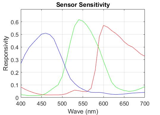
There are two important types of data that are necessary for this project, spectral radiance measurements and raw camera images. To gather the data, a Macbeth ColorChecker is illuminated by a known illuminant. The radiance measurements can then be taken using a spectrophotometer (in this case the Photoresearch spectrophotometer, model PR670 was used). This is considered the input of the camera. The Google Pixel 4A is used to capture the camera output (i.e. the images). These images are the digital negative values (DNG) files. This phone uses the Sony IMX363 sensor, which is well documented. Sony has published the sensor's spectral sensitivity data and it has previously been input in ISETCAM, shown in Figure 1. This will be helpful to compare our model with.
Since this project creates and tests the model, we have "training" datasets and test datasets. The former are referred to as Measurements1 and the latter, Measurements2. Measurements1 contains radiance data and DNG files for the MCC illuminated by one of three illuminants, Tungsten (A), Cool White Fluorescent (CWF), and Daylight (DAY). Measurements2 contains radiance data and DNG files for the MCC illuminated by a Tungsten light. All the camera images are taken with the same ISO Speed, but have different Exposure Times.
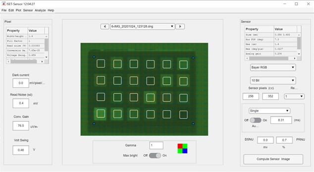
We have to extract the RGB values from the DNG files. For this, we use ISETCAM's sensor functions. First we read the DNG file using sensorDNGRead. Then we open a window that displays the sensor image using, sensorWindow.From there we estimate rectangles where the 24 boxes are on the MCC using the chartCornerpoints function. An example of the sensor window with the rectangles charted is shown in Figure 2. If we are satisfied by the placement of the rectangles, we get the digital values from each square using the function chartRectsData. We then get the mean and standard deviation of the RGB values for each square. The RGB mean values have to be corrected for Black Level and Exposure Time. This is done by subtracting the Black Level, then dividing the difference by the exposure durations. This is especially important if the exposure durations for the images are different.
Making the Spectral QE Model
This project utilizes multiple methods to improve the spectral quantum efficiency model.
Simple Linear Equation
To solve for the spectral quantum efficiency matrix, the previously explained linear equation was used. However, doing this alone is not sufficient to get an accurate model. This is the case, in part, because the radiance data was generated by measuring the radiance of MCC. Our data technically has 72 samples (24 per MCC x 3 illuminants), but the patches are not independent. As we'll see, in the coming sections, there is less than 10 independent measurements in our radiance dataset. Since we are trying to get the spectral QE information for 31 wavelengths (400:10:700 nm), we are heavily under-sampled.
Furthermore, simply solving the linear equation will create an overfitted model.
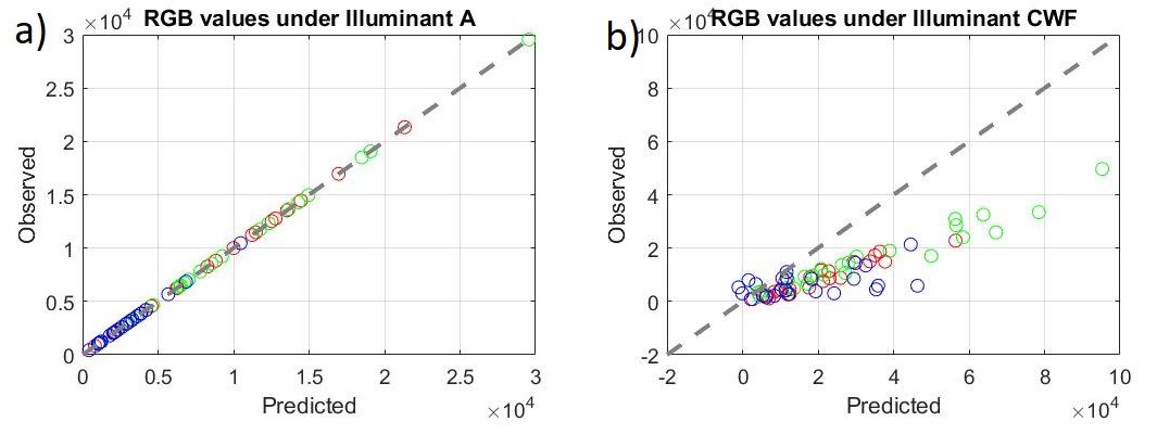
For example, the spectral QE was solved for with the subset of the radiance data for which the MCC is illuminated by a Tungsten light. This spectral QE can be used to predict the observed RGB values for this illumination with 0 error. However, this model does a very poor job of predicting the observed RGB values for a different illumination, with an rms error over 1. These results are shown in Figure 2. One way of fixing this is using only a few of the most important principal components. This is discussed in the next section.
Lower Dimensional Model
There are multiple ways of solving for the principal components of the radiance data. In this work, Singular Value Decomposition (SVD) was used. Performing SVD on the radiance data outputs 3 matrices, U, S, V. We can use D to calculate the variance of the dataset. We use the Matlab cumsum function to find the cumulative sum of the elements along the diagonal of D. We then divide the cumulative sum by the sum of D. When this operation equals 1, all of the variation of the dataset is within that subset of the data. When this is close to zero, it means that very little of the variation is represented in that subset of the data. When performing this operation on the radiance data from Measurements1, we get the plot shown in Figure 3. We can see that as more columns of 'D' are included in the sum, the proportion of variation is almost 1 when about 10 columns of D are included in the sum. To prevent overfitting, we want to include the principal components that account for less than 0.95 of the variation. In our case, this is with less than 8 principal components.

Now that we know how many principal components to include in our low-dimensional model, we can represent it as a weighted sum of those components,
For our new basis, we use some amount of the most important principal components. We get these principal components from left singular vector, U. For example, if we let p be the number of principal components we will use, then our new basis is
As explained in the previous section, we want to choose a p such that proportion of variation represented in the dataset is less that 0.95, but we do not want to choose something with too little variation represented. In this work, p = 6 is chosen.
Now, we can solve for the weights:
While there are many ways to calculate the inverse of a matrix in Matlab, the pseudoinverse (pinv) was chosen because it saves computing time, and outputs a reasonably accurate inverse.
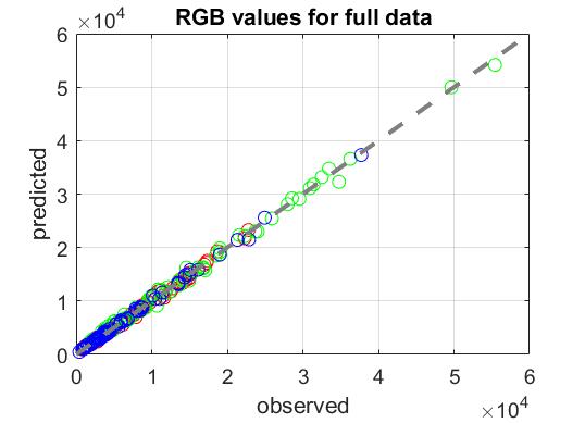
The spectral QE can then be calculated with the basis and weights to give us a low-dimensional model. The low-dimensional model does not have a problem with overfitting. To check this, the model was made with the full radiance dataset. Then the model predicted the RGB values. The results when compared to the observed values are shown in Figure 4. Here, the rms error was 0.04. A good metric to compare the rms error to is the standard deviation of the dataset, which in our case was 0.051. These values are quite close together, making this a good approximation.
Best Linear Fit
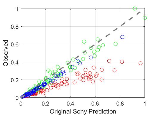
When comparing the observed RGB values with the RGB values predicted by Sony's spectral QE model, there is quite a bit of error, 0.39. This is shown in Figure 5. Notice that particularly the red channel is off. This discrepancy between Sony's characterization and what is observed could be because of mixing between channels and channel gains being off.
We can fit the Sony model to our observed data by a linear transformation, L:
Now to get the fitted Sony spectral quantum efficiency we just multiply the original Sony curves by the linear transformation L:
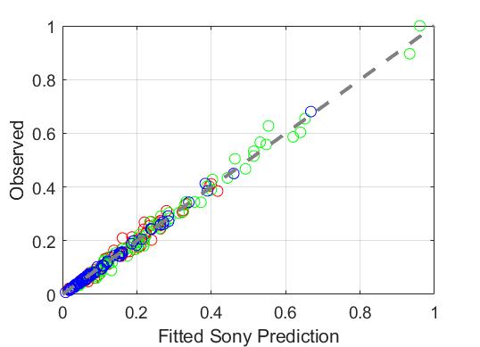
Now, re-predicting the RGB values with the fitted Sony Spectral QE, the error is much lower, 0.066. The results of this re-prediction are shown in Figure 6.
Testing the Model
Once we are confident in our model, we can test it with a new dataset, Measurements 2.
First we read the radiance data and extract the RGB values from the DNG files. Then we use our low-dimensional model on the new radiance data to predict the RGB values. We compare the predicted and observed RGB values. We can also compare these values with the predictions of the Sony model and calculate the RMS error.
Results
Sony Linear Fit and Our Estimate
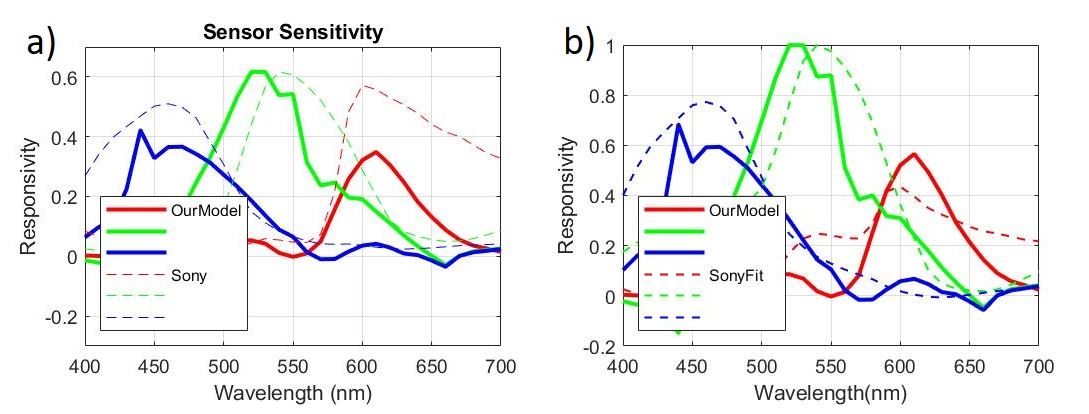
After completing all the previous steps, we have a Spectral QE model and a linearly fitted Sony Spectral QE that we can use on the new radiance dataset from Measurements2. Figure 7 shows our low-dimensional model compared to the original (a) and fitted (b) Sony spectral QE model. The most obvious change between the original and linearly fit Sony models is in the red channel. In the original, the red channel has a much higher peak responsivity than our estimate. The opposite is true in comparison to the fitted model.
RGB Value Comparisons and Error
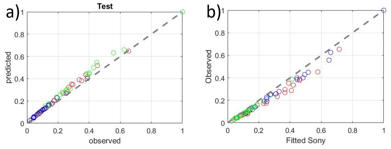
The final results are the outcome when comparing the predicted and observed RGB values for the Measurements2 data, shown in Figure 8. The rms error between the observed RGB values and those predicted by the fitted Sony model is 0.153. The error between the observed RGB values and those predicted by our low-dimensional model is 0.126. So while our estimate is slightly better than the fitted Sony model, both are similar in accuracy.
Conclusions
This project provides a good model for predicting RGB values using radiance data. However, there are many ways this work can be built upon. The model could be tested on more datasets and improved from there. Additionally, one could deal more exactly with the problem of overfitting. In this work, a basis was chosen to be less than 8 principal components and to minimize the error when testing the model. However, someone could more closely analyze the data to determine exactly when overfitting starts to occur. The majority of this work was making the model using the full radiance dataset from Measurements1. In the future, someone could explore how accurately the model would be using the data from just one illuminant to train it. Would it be just as accurate when tested on data from a different illuminant as it is when tested on data from same illuminant? Additionally, the project can be modified to predict the CIELAB color image metrics.
Prior to completing this project, I did not have a lot of experience in data analysis. I have learned to identify whether a model is overfitted and whether the data is undersampled. Furthermore, I learned techniques about how to deal with these problems. Learning to calculate the proportion of the variation in a subset of a dataset was particularly helpful to my understanding of the problems with the results of the simple linear equation. In the past I was only exposed to singular value decomposition from a mathematical/theoretical perspective, so it was satisfying to use it as an engineering tool. I am pleased to say that after completing this project my understanding of how to use ISETCAM to model the image processing pipeline has deepened and I am more confident in my ability to use the program in the future.
References
- Soft prototyping imaging systems for oral cancer. J. Farrell, Z. Lyu, Z. Liu, H. Blasinski, Z. Xu, J. Rong, F. Xiao, B. Wandell.
- Digital camera simulation (2012). J. E. Farrell, P. B. Catrysse, B.A. Wandell . Applied Optics Vol. 51 , Iss. 4, pp. A80–A90
- Linear Models of Surface and Illuminant Spectra (1992). D. H. Marimont, B.A. Wandell. Journal of the Optical Society of America A Vol. 9, Iss. 11, pp. 1905
- A Comparison of Methods of Sensor Spectral Sensitivity Estimation (1994). P.M. Hubel, D. Sherman, J. E. Farrell.
- Overfitting Definition
- Singular value decomposition. (2020, November 09). Retrieved November 27, 2020
- Dimension Reduction(2020, May 01). R. Peng. Retrieved November 27, 2020
Appendix: Source Code
Saved in this Google Drive is the main source code: ColorCalibration.mlx. There are two folders, Measurements1 and Measurements2, which contain the training and testing data, respectively. Within each of these folders contains a set of Spectral Radiance Measurements and DNG Files.
Acknowledgements
Thank you to all the instructors of Psych221 for an interesting class this past quarter. A special thank you to Professor Farrell and Professor Wandell for taking all the data needed to complete this project and for their guidance the past couple of weeks.