WooLee: Difference between revisions
imported>Projects221 |
imported>Projects221 |
||
| (4 intermediate revisions by the same user not shown) | |||
| Line 101: | Line 101: | ||
We decide to try simple 3D reconstruction. We will use 2 images: one is original image, the other is shifted image of the original one. By using two images mentioned above, we can get a depth that that could be used in 3D reconstruction. From the 2D images and for each certain portion we check how that portion is close to the portions in the other image. | We decide to try simple 3D reconstruction. We will use 2 images: one is original image, the other is shifted image of the original one. By using two images mentioned above, we can get a depth that that could be used in 3D reconstruction. From the 2D images and for each certain portion we check how that portion is close to the portions in the other image. | ||
==== Method 1: Autocorrelation ==== | ==== Method 1: Autocorrelation ==== | ||
3D reconstruction can be done by using the concept of autocorrelation. The highest value of the autocorrelation is always the multiplication of itself, meaning the same image portion in our case. We fix the position of the portion in the original figure and move that in the second figure to compute the autocorrelation. For this computation we also include normalized constant to take weight into account. Once the highest value of the autocorrelation is found we select that that position of the second image corresponds to that of the first image. | 3D reconstruction can be done by using the concept of autocorrelation. The highest value of the autocorrelation is always the multiplication of itself, meaning the same image portion in our case[Miao]. We fix the position of the portion in the original figure and move that in the second figure to compute the autocorrelation. For this computation we also include normalized constant to take weight into account. Once the highest value of the autocorrelation is found we select that that position of the second image corresponds to that of the first image. | ||
==== Method 2: Subtraction ==== | ==== Method 2: Subtraction ==== | ||
Another approach is we subtract the image portion of original to that of the other. And then sum all the values computed. Other than this we do the same procedure: move the portion of the second image and compute the subtraction (also normalization is included here). In this case, however, the lowest values will let us know the position of the second image that corresponds to that of the first image. | Another approach is we subtract the image portion of original to that of the other. And then sum all the values computed [Leens]. Other than this we do the same procedure: move the portion of the second image and compute the subtraction (also normalization is included here). In this case, however, the lowest values will let us know the position of the second image that corresponds to that of the first image. | ||
==== Generate 3D depth Map ==== | ==== Generate 3D depth Map ==== | ||
We can measure the distance of the positions. If an object is further from the camera views, the distance would be short. If an object is close to the camera views, the distance would be long. From this we can generate depth-map plot, giving high values to close objects and low values to distant objects. | We can measure the distance of the positions. If an object is further from the camera views, the distance would be short. If an object is close to the camera views, the distance would be long. From this we can generate depth-map plot, giving high values to close objects and low values to distant objects. | ||
| Line 120: | Line 120: | ||
The figure below shows the conversion of 3D objects to a 3D scene. The figure on the right hand side below shows the PBRT-converted 3D scene from 3D objects in the figure on the left hand. | The figure below shows the conversion of 3D objects to a 3D scene. The figure on the right hand side below shows the PBRT-converted 3D scene from 3D objects in the figure on the left hand. | ||
<br> | <br> | ||
[[File:ObjectPbrt.png |thumb|500px|center| Figure 9 Object | [[File:ObjectPbrt.png |thumb|500px|center| Figure 9 Object PBRT]] | ||
<br> | <br> | ||
In PBRT exporter in Blender, we are able to set up the objects. We control the texture, material types, diffusion, etc. We configured as much as possible to mimic the 3D scene as close as the 3D initial objects. | In PBRT exporter in Blender, we are able to set up the objects. We control the texture, material types, diffusion, etc. We configured as much as possible to mimic the 3D scene as close as the 3D initial objects. | ||
| Line 133: | Line 133: | ||
We have coded 2 methods and tried to reconstruct the 3D depth using two files(codes attached in Data: slprac_ files). Following figure shows the result of the depth map plot. | We have coded 2 methods and tried to reconstruct the 3D depth using two files(codes attached in Data: slprac_ files). Following figure shows the result of the depth map plot. | ||
[[File:3DDepthResult.png |thumb|500px|center| Figure 11 3D Depth result]] | [[File:3DDepthResult.png |thumb|500px|center| Figure 11 3D Depth result]] | ||
From the figures we see that the depth map has not been generated well. Comparing to the 3D depth map ground truth, we realize that our result is not comparable to the reference value. This is because we do not have the initial depth math information about the scene. The backgrounds of two image do not change much at all. Thus, the result we have gotten represents the relative depth value. In order to get 3D depth map accurately, we need to have intial depth information to begin with | From the figures we see that the depth map has not been generated well. Comparing to the 3D depth map ground truth, we realize that our result is not comparable to the reference value. This is because we do not have the initial depth math information about the scene. The backgrounds of two image do not change much at all. Thus, the result we have gotten represents the relative depth value. In order to get 3D depth map accurately, we need to have intial depth information to begin with [Scharstein]. | ||
= Conclusions = | = Conclusions = | ||
| Line 143: | Line 143: | ||
== From 3D scenes to 3D objects == | == From 3D scenes to 3D objects == | ||
For 3D reconstruction, initially, the parallel shifted picture of original picture was gotten correctly. The algorithm that we decide to use lack in information as we assume that we do not have initial depth information about the 3D scenes. We could have improved the result, even without having the information about the depth, if we use larger portion, such as a square window for comparing the image matching computation | For 3D reconstruction, initially, the parallel shifted picture of original picture was gotten correctly. The algorithm that we decide to use lack in information as we assume that we do not have initial depth information about the 3D scenes. We could have improved the result, even without having the information about the depth, if we use larger portion, such as a square window for comparing the image matching computation. Perhaps, we could assume that the depth is getting deeper from the bottom to the top of the image as it is what a camera normally look through. | ||
== Limitations == | == Limitations == | ||
| Line 160: | Line 160: | ||
=== PBRT === | === PBRT === | ||
<br> | <br> | ||
PBRT: www.pbrt.org | |||
<br> | <br> | ||
=== Computer Vision === | === Computer Vision === | ||
Scharstein and Szeliski(2002). "A Taxonomy and Evaluation of Dense Two-Frame Stereo Correspondence Algorithms". International Journal of Computer Vision 47: 7-42. | Scharstein and Szeliski(2002). "A Taxonomy and Evaluation of Dense Two-Frame Stereo Correspondence Algorithms". International Journal of Computer Vision 47: 7-42. | ||
| Line 171: | Line 172: | ||
= Appendix I - Code and Data = | = Appendix I - Code and Data = | ||
== | ==Data with Codes== | ||
The following file contains all the data and codes that we have made and utilized. | |||
<br> | |||
[[File:Scene3DMatlab.zip]] | [[File:Scene3DMatlab.zip]] | ||
= Appendix II - Work partition (if a group project) = | = Appendix II - Work partition (if a group project) = | ||
Latest revision as of 07:22, 21 March 2013
Back to Psych 221 Projects 2013
Background
It is no wonder that vision is one of the most important parts in our lives. Besides, due to the tremendous improvements in technology, research on 3D vision has become hot topic. 3D reconstruction is interesting in a way that we could realize a 3D image by just looking at a 2D image. In this project, we provide some techniques for developing scene models that could be used in analysis in ISET. We build the scene using Blender and export it to PBRT files. Then, in Matlab, we run the ISET to analyze the scene converted. We also attempted to do 3D reconstruction, demonstrating a possible way of using scenes for computer vision testing.
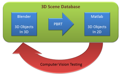
Blender
Blender allows us to design 3D objects in 3D space. It has various features, such as modeling, texturing, lighting, animation and video post-processing functionality. Also, it is highly compatible with other files so that we can make use of other 3D files to edit them. The figure below shows basic Blender interfaces.
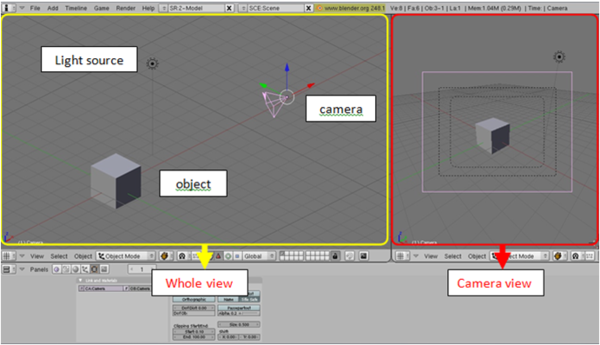
Take a cube as an example as shown fig.x. There is an object, which is a cube in this example, light source, and camera. On the left side of the figure.x, it shows whole scene that we created, on the right side, it shows the scene which is viewed through the camera. We can control the parameters and the properties of those; - object : edit geometry, size of the object, control reflectance such as diffuse, specular - light source : set light source as you would like to use such as D65 - camera : viewing position, choose lens
PBRT
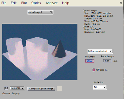
PBRT stands for Physically Based Rendering Tool, and it is a render for graphics. It does not have any specific interface like Blender. Of various functions, transferring a 3D image data of an object to a 2D image data is the function that we are looking for. PBRT is a powerful that it can store the 2D data as if we take a picture of a 3D object. It takes point of view, reflectance, shades, etc. into account when converting. Below shows the converted 2D picture from 3D objects.
Methods
Using Blender to Create Scenes
In our project, Blender is used for creating scene. In our case, we must use the version 2.48a. There are few steps to do this.
import the file
Import the file which is filename.dae.
texturing
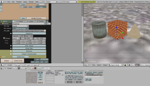
To make texture on the object, texture image is needed, and it should be converted to .tga format. Then we put the texture image on the object. Also, we can apply the material to the object using texture menu shown in the figure.
control reflectance
We are able to control reflectance, light source as well. In the case of reflectance, it is allowed to apply diffuse and specular reflectance on the object.
export to pbrt
Finally, the scene has been created by exporting the image to pbrt using exporter. Go to render menu, and click the export to pbrt.
Here are some examples of 3D objects created via Blender.

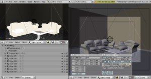

Using PBRT to create 3D scene
Set up
First of all, we need to initialize ISET and configure some files to make PBRT work. Go to the corresponding ISET directory in Matlab and type:
>> isetPath(pwd)
>> ISET
We have used scene3Dmatlab directory (downloadable). In that directory type:
>> addpath(genpath(pwd))
Now, we are ready to use PBRT.
PBRT files
From the exporter in Blender, we achieve several files. Those are default.pbrt, default-geom.pbrt, and default-mat.pbrt (default-vol.pbrt is not used, and the name default can be changed). Brief descriptions are below:
- default.pbrt : includes camera lens information, sampling pixels
- default-geom.pbrt : includes the geometry of the objects
- default-mat.pbrt : includes the information for the material such as texture
Some files, if necessary, need to be changed, such as file paths for texture and minor settings (number of sampling pixels, camera position, etc).
Run PBRT
We can execute PBRT in a command line, but we prefer to use Matlab because we could make coding neat and use features in Matlab in order to analyze PBRT files. The following is the code we used:
chdir(fullfile(s3dRootPath, 'scripts', 'pbrtFiles'));
unix([fullfile(pbrtHome, '/src/bin/pbrt ') 'default.pbrt']); # generate PBRT to make images
oi = pbrt2oi('output.dat');
vcAddAndSelectObject(oi);
oiWindow;
m = oiGet(oi, 'mean illuminance')
We can open this output with ISET. Other detailed codes are attached in the references With this image files we can now consider doing some computer vision testing.
Computer Vision Testing: 3D depth reconstruction
Ideas for 3D depth reconstruction
We decide to try simple 3D reconstruction. We will use 2 images: one is original image, the other is shifted image of the original one. By using two images mentioned above, we can get a depth that that could be used in 3D reconstruction. From the 2D images and for each certain portion we check how that portion is close to the portions in the other image.
Method 1: Autocorrelation
3D reconstruction can be done by using the concept of autocorrelation. The highest value of the autocorrelation is always the multiplication of itself, meaning the same image portion in our case[Miao]. We fix the position of the portion in the original figure and move that in the second figure to compute the autocorrelation. For this computation we also include normalized constant to take weight into account. Once the highest value of the autocorrelation is found we select that that position of the second image corresponds to that of the first image.
Method 2: Subtraction
Another approach is we subtract the image portion of original to that of the other. And then sum all the values computed [Leens]. Other than this we do the same procedure: move the portion of the second image and compute the subtraction (also normalization is included here). In this case, however, the lowest values will let us know the position of the second image that corresponds to that of the first image.
Generate 3D depth Map
We can measure the distance of the positions. If an object is further from the camera views, the distance would be short. If an object is close to the camera views, the distance would be long. From this we can generate depth-map plot, giving high values to close objects and low values to distant objects.
Generating two 2D camera view images
In order to do 3D reconstruction. We need two images, and the viewpoints of them need to share at least one axis and perpendicular to the viewing direction. After exporting from Blender to PBRT, we can create another PBRT file viewing from another perspective by adjusting LookAt in default.pbrt. Utilizing the concept of linear algebra, we can deduce the points for the second camera. This way we would avoid uncertain error made in Blender because the computation of such point would be much more accurate than moving a camera. The following figure shows the vector of the camera.

We know the two points consisting of the direction vector of the first camera. Using those points, we can get the vector points for the second camera.
Results
From Blender to PBRT
The figure below shows the conversion of 3D objects to a 3D scene. The figure on the right hand side below shows the PBRT-converted 3D scene from 3D objects in the figure on the left hand.
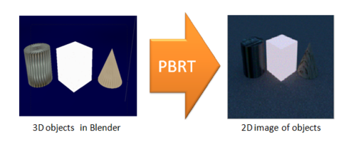
In PBRT exporter in Blender, we are able to set up the objects. We control the texture, material types, diffusion, etc. We configured as much as possible to mimic the 3D scene as close as the 3D initial objects.
3D depth map ground truth
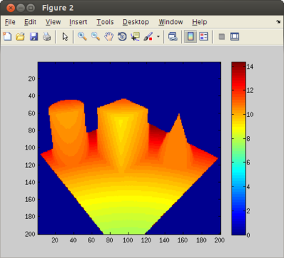
We generated 3D depth map ground truth plot, which is the theoretical values of the 3D depth(s_s2dRenderDepthMapExample.m). This can be useful to compter vision testing since it could be the reference values for 3D depth reconstruction. As an example, we attach the result of the 3D depth map ground truth for the 3 objects we created.
3D depth recontruction
We have coded 2 methods and tried to reconstruct the 3D depth using two files(codes attached in Data: slprac_ files). Following figure shows the result of the depth map plot.
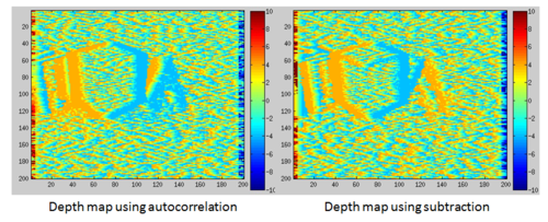
From the figures we see that the depth map has not been generated well. Comparing to the 3D depth map ground truth, we realize that our result is not comparable to the reference value. This is because we do not have the initial depth math information about the scene. The backgrounds of two image do not change much at all. Thus, the result we have gotten represents the relative depth value. In order to get 3D depth map accurately, we need to have intial depth information to begin with [Scharstein].
Conclusions
The purpose of our project is to provide 3D scene database for computer vision testing. One object is to show various 3D objects can be created and provide 3D scenes by converting 3D objects to 3D scene (2D image file). After this is done. We demonstrated how these generated images can be used to computer vision testing. A little change in the camera position in PBRT file allows us to get another image that is shifted from the original image. This way we were able to work on 3D depth reconstruction.
From 3D objects to 3D scene
If we use various feature provided in Blender, we can easily generate 3D objects that are quite detailed and complicated. However, Blender is a heavy tool that requires many skills from users to utilize it well. We can still generate relatively detailed object via importing. The camera view in Blender is the 3D object models created while the result from PBRT is the real camera view that takes things like reflectance, shade, diffusion, etc. into account; thus, the camera view in Blender cannot be very close to the 2D image of 3D scene.
From 3D scenes to 3D objects
For 3D reconstruction, initially, the parallel shifted picture of original picture was gotten correctly. The algorithm that we decide to use lack in information as we assume that we do not have initial depth information about the 3D scenes. We could have improved the result, even without having the information about the depth, if we use larger portion, such as a square window for comparing the image matching computation. Perhaps, we could assume that the depth is getting deeper from the bottom to the top of the image as it is what a camera normally look through.
Limitations
There are many things that we would like to do next in order to improve our work. We had technology issues when we were doing project. Most of all, the computer we have does not have high performance, though it works quite well for mundane purposes (like word processing and other programming). Blender is a big tool to manipulate 3D objects and has many features. Furthermore, when we also ran Matlab to use PBRT and ISET (running in different OS's), the computer became very slow, (and this slowed down our progress). With more memory, we would overcome this issue and try various things. When we would like to generate 3D scene, the initial setup time cost is quite large (about 1 hour), and for each time modifying it takes about half an hour. For some images, converting to 3D scene via PBRT takes more than an hour. If this process can be abridged, we would have more time to analyze and debug.
Future works
This project opens many possibilities for the future works. First of all, in Blender, we could study more features in Blender to create more realistic objects. By understanding more profoundly about the PBRT exporters, we could control the qualities of the 3D scenes. Furthermore, we can manipulate PBRT files to make the images more detailed and accurate. We could model better version of camera to get more rendered images. Finally, many things could be done in computer vision testings. For 3D reconstruction, we would like to work on generating more accurate 3D depth map.
Blender
http://wiki.blender.org/index.php/
http://wiki.blender.org/index.php/Doc:2.4/Manual/Introduction
PBRT
PBRT: www.pbrt.org
Computer Vision
Scharstein and Szeliski(2002). "A Taxonomy and Evaluation of Dense Two-Frame Stereo Correspondence Algorithms". International Journal of Computer Vision 47: 7-42.
Miao and Chen. "2nd Response to 'Feasibility of 3D reconstruction from a single 2D diffraction measurement" Retrieved from arxiv.org/pdf/0910.0272
Leens et al(2009). "Combining Color, Depth, and Motion for Video Segmentation." ICVS 2009.
Appendix I - Code and Data
Data with Codes
The following file contains all the data and codes that we have made and utilized.
File:Scene3DMatlab.zip
Appendix II - Work partition (if a group project)
We work closely together all the time almost everyday since we had started our project. For each part we all work together as well so it is difficult to partition. Roughly, for the preparation for the presentation,
Seul - worked on Blender, computer vision debugging
Seung Je - worked on PBRT rendering, computer vision algorithm coding
We also got lots of helpful advice from Andy Lai Lin.