Depth Mapping Algorithm Performance Analysis

Introduction

We will implement various disparity estimation algorithms and compare their performance.

Background

Disparity and Depth

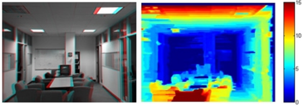
Depth information about a scene can be captured using a stereo camera (2 cameras that are separated horizontally but aligned vertically). The stereo image pair taken by the stereo camera contains this depth information in the horizontal differences (when comparing the stereo image pair, objects closer to the camera will be more horizontally displaced). These differences (also called disparities) can be used to determine the relative distance from the camera for different objects in the scene. In Figure 1, you can see such differences on the left where the red and blue don't match up.

Figure 1. Anaglyph of stereo image pair (left) and example disparity map computed from the same stereo image pair (right)

Disparity and depth can be related by the following equation (where x-x' is disparity, z is depth, f is the focal length, and B is the interocular distance). !!!!!!!!!!!!OSCAR WRITE STUFF HERE!!!!!!!!!!!!!!!!!!!!!!

$x-x'={\frac {Bf}{z}}$

Figure 2. Diagram to Calculate Disparity and Depth

Image Rectification

In order to extract depth information, the stereo image pair must first be rectified (i.e. the images must be transformed in some way such that the only differences that remain are horizontal differences corresponding to the distance of the object from the camera). Rectification can be accomplished both with and without camera calibration.

If the corresponding camera intrinsics and extrinsics are given for the stereo image pair, then calibration is not necessary. If they are not given, but photos of a checkerboard or some other calibration object are provided, then the calibration parameters can be calculated. !!!!!!!!!!!!!!!!!!!!TALK ABOUT CALIBRATED RECTIFICATION HERE??????!!!!!!!!!!!!!!1

If not enough camera parameters are given and there are no checkerboard images to be used for calibration, then the following 4 steps can be used for rectification of a given stereo image pair.

• First we detect SURF keypoints (a scale and rotation invariant feature detector) in each stereo image and extract the feature vectors of each keypoint.
• We then find matching keypoints between the images using a similarity metric. The uncalibrated rectification used by MATLAB uses the sum of absolute differences metric.
• We then remove outliers (incorrect matches) using an epipolar constraint. Looking at Figure 3, this means that for a keypoint x on the left image, the matching keypoint on the right image must lie on the corresponding epipolar line defined by the intersection of the epipolar plane and the image plane.
• Now using the vector distance between the remaining correct matches, we must compute a 2D projective geometric transformation to apply to one or both of the stereo images. After transformation, the stereo images should no longer have any vertical displacement.

Figure 3. Applying epipolar constraint to keypoint matches.

Results

Reference image

Sum of Squared Differences

Disparity Map from SSD

Sum of Absolute Difference

• Performance with default parameters

Disparity Map without semi-global matching

Disparity Map with semi-global matching

• Effect of Block Size and Smoothing

For block matching with and without the semi-global smoothing, we tested the effect of altering the block size of the Block Matching + SAD algorithm. The chart below shows the resulting error rates, along with the corresponding graph.

Census Transformation

Disparity Map from Census Transformation

Appendix II

We divided the work as follows:

• Oscar Guerrero:
• Deepti Mahajan:
• Shalini Ranmuthu:

You can write math equations as follows: $y=x+5$

You can include images as follows (you will need to upload the image first using the toolbox on the left bar.):

caption