Depth Mapping Algorithm Performance Analysis

Introduction

We will implement various disparity estimation algorithms and compare their performance. ADD MORE

Background

Disparity and Depth

Depth information about a scene can be captured using a stereo camera (2 cameras that are separated horizontally but aligned vertically). The stereo image pair taken by the stereo camera contains this depth information in the horizontal differences (when comparing the stereo image pair, objects closer to the camera will be more horizontally displaced). These differences (also called disparities) can be used to determine the relative distance from the camera for different objects in the scene. In Figure 1, you can see such differences on the left where the red and blue don't match up.

Figure 1. Anaglyph of stereo image pair (left) and example disparity map computed from the same stereo image pair (right)

Disparity and depth can be related by the following equation (where x-x' is disparity, z is depth, f is the focal length, and B is the interocular distance). !!!!!!!!!!!!OSCAR/SHALINI WRITE STUFF HERE!!!!!!!!!!!!!!!!!!!!!!

$x-x'={\frac {Bf}{z}}$

Figure 2. Diagram to Calculate Disparity and Depth

Image Rectification

In order to extract depth information, the stereo image pair must first be rectified (i.e. the images must be transformed in some way such that the only differences that remain are horizontal differences corresponding to the distance of the object from the camera). Rectification can be accomplished both with and without camera calibration. If the corresponding camera intrinsics and extrinsics are given for the stereo image pair, then calibration is not necessary. If they are not given, but photos of a checkerboard or some other calibration object are provided, then the calibration parameters can be calculated.

If not enough camera parameters are given and there are no checkerboard images to be used for calibration, then the following 4 steps can be used for rectification of a given stereo image pair.

• First we detect SURF keypoints (a scale and rotation invariant feature detector) in each stereo image and extract the feature vectors of each keypoint.
• We then find matching keypoints between the images using a similarity metric. The uncalibrated rectification used by MATLAB uses the sum of absolute differences metric.
• We then remove outliers (incorrect matches) using an epipolar constraint. Looking at Figure 3, this means that for a keypoint x on the left image, the matching keypoint on the right image must lie on the corresponding epipolar line defined by the intersection of the epipolar plane and the image plane.
• Now using the vector distance between the remaining correct matches, we must compute a 2D projective geometric transformation to apply to one or both of the stereo images. After transformation, the stereo images should no longer have any vertical displacement.

Figure 3. Applying epipolar constraint to keypoint matches.

Datasets

SYNS Dataset

 !!!!SHALINI FIX THIS!!!!

The Southampton-York Natural Scenes (SYNS) dataset contains image and 3D range data measured from different rural and urban locations. Each sample contains the following data:

• LiDAR depth information (360 x 135 degree field of view)
• Panoramic HDR image captured with a SpheroCam (Nikkor fish-eye lens) (360 x 180 degree image)
• Stereo image pairs captured with 2 Nikon DSLR cameras (each image pair was captured at a different rotation of the camera such that all of them covered a 360 degree view of the surroundings)

No intrinsics/extrinsics or calibration data → use uncalibrated rectification on stereo images → compute depth map

Figure 4. Stereo images rectified with uncalibrated rectification.

Figure 5. Disparity map computed from rectified stereo images in Fig. 4.

Want to compare depth map to LiDAR info (ground truth) Use SYNS script to scale panoramic LiDAR info to panoramic HDR image Least mean squares algorithm to map rectified stereo images to the panoramic HDR and find region of interest Extract corresponding LiDAR info and compare to computed depth map

Figure 6. LiDAR info (left) mapped to HDR panorama (right)

Middlebury Dataset

The Middlebury Data set was created by Nera Nesic, Porter Westling, Xi Wang, York Kitajima, Greg Krathwohl, and Daniel Scharstein at Middlebury College during 2011-2013, and refined with Heiko Hirschmüller at the DLR Germany during 2014.

Methods: Similarity Metrics

SAD

The sum of absolute differences (SAD) is a measure of the similarity between image blocks. It is calculated by taking the absolute difference between each pixel in the original block and the corresponding pixel in the block being used for comparison. [3]

• Compute the difference and sum over all pixels

  

SSD

The sum of squared difference takes the squared differences within the two blocks. This measure has a higher computational complexity compared to SAD algorithm as it involves numerous multiplication operations. [3]

• Compute the squared difference and sum over all pixels

NCC

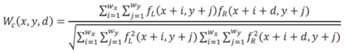
Normalized cross-correlation is a metric to evaluate the degree of similarity (or dissimilarity) between two compared images. In NCC, a window of suitable size is determined and moved over the entire image or the cost matrix. The correspondence is thus obtained by dividing the normalized summation of the product of intensities over the entire window by the standard deviation of the intensities of the images over the entire window. [3]

• Compute the cross-correlation

  

CT

The census transform encodes the relative brightness of each pixel (with respect to its neighbors) and compares the digital encoding of pixels from windows from each image (left and right). The algorithm is as follows:

• Compute bit-string for pixel p, based on intensities of neighboring pixels

• Compare left image bit-string with bit-strings from a range of windows in the right image

• Choose disparity d with lowest Hamming distance

Methods: Algorithm Evaluation

Talk about

• Tried these 3 algorithms, x pictures for each
• How error rate is calculated and/or averaged
• Other stuff

Results

Reference image

Sum of Squared Differences

Disparity Map from SSD

Sum of Absolute Difference

Performance with default parameters

Disparity Map without semi-global matching

Disparity Map with semi-global matching

Effect of Block Size and Smoothing

For block matching with and without the semi-global smoothing, we tested the effect of altering the block size of the Block Matching + SAD algorithm. The chart below shows the resulting average error rates over 15 images, along with the corresponding graph.

Overall, the semi-global smoothing had a significantly lower error rate than regular SAD. Furthermore, the block size affects the performance of each differently -- semi-global SAD produces lower error rates with smaller block sizes, and SAD has a local optimum around a block size of 11.

Comparing the computational time of each algorithm over all block sizes tested, SAD with semi-global smoothing took an average of 0.9598 seconds per image, while SAD took an average of 0.3016 seconds. Thus, regular SAD is more than three times as fast.

Census Transformation

Disparity Map from Census Transformation

Conclusions

Available Datasets

!!!!!SHALINI DO THIS!!!!!

References

[1] Daniel Scharstein, et. al., “High-Resolution Stereo Datasets with Subpixel-Accurate Ground Truth” German Conference on Pattern Recognition. 2014. http://www.cs.middlebury.edu/~schar/papers/datasets-gcpr2014.pdf

[2] Jongchul Lee, et. al., "Improved census transform for noise robust stereo matching," Optical Engineering 55(6), 063107 (16 June 2016). http://dx.doi.org/10.1117/1.OE.55.6.063107

[3] Pranoti Dhole, et. al., "Depth Map Estimation Using SIMULINK Tool," 3rd International Conference on Signal Processing and Integrated Networks. 2016.http://ieeexplore.ieee.org/stamp/stamp.jsp?arnumber=7566714

Appendix I

• MATLAB code for disparity map algorithms and evaluation code: File:Projectcode.zip
• Link to Middlebury dataset: http://vision.middlebury.edu/stereo/data/scenes2014/
• Link to SYNS dataset: https://syns.soton.ac.uk/

Appendix II

We divided the work as follows:

• Oscar Guerrero:
• Deepti Mahajan: Implemented algorithms, ran experiments and gathered results, worked on presentation and wiki
• Shalini Ranmuthu:

You can write math equations as follows: $y=x+5$

You can include images as follows (you will need to upload the image first using the toolbox on the left bar.):

caption