Neuroimaging: Difference between revisions
imported>Projects221 |
imported>Projects221 |
||
| Line 95: | Line 95: | ||
>90% similarity = MRIs of the same brain<br> | >90% similarity = MRIs of the same brain<br> | ||
==== Explanation ==== | ==== Explanation ==== | ||
The main deterministic factor in the brain matching algorithm is the cross correlation. The files are three dimensional vectors; hence a three dimensional cross correlation is needed. But certain steps are taken to try and ensure a meaningful cross correlation is taken: | |||
1. First two or more files must be selected from the NIFTI database given. | 1. First two or more files must be selected from the NIFTI database given. | ||
2. In order to calculate the cross correlation the Fourier transform of each file is needed. Using functions such as ‘fftn’ and ‘fftshift,’ the Fourier transform of each file is taken. | 2. In order to calculate the cross correlation the Fourier transform of each file is needed. Using functions such as ‘fftn’ and ‘fftshift,’ the Fourier transform of each file is taken. | ||
3. Cross-correlation | 3. Cross-correlation | ||
i. The cross correlation is simply multiplying the Fourier transform of one file by the conjugate of the Fourier transform of the second file. This then returns a non-normalized single value that is characteristic of how | i. The maximum value of the cross-correlation is simply multiplying the Fourier transform of one file by the conjugate of the Fourier transform of the second file and then determining the maximum value. This then returns a non-normalized single value that is characteristic of how well the maximum value their image alike. | ||
3. In order to normalize the cross-correlation, the | 3. In order to normalize the cross-correlation, the product of the sum of the all the pixel intensities was taken. Then each maximum value from the cross-correlation was divided by the product of the sum of the vectors. This allows for the maximum value of the cross-correlation of an image with itself to be one. | ||
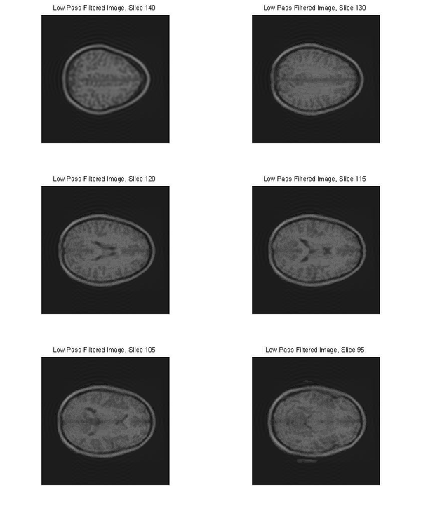
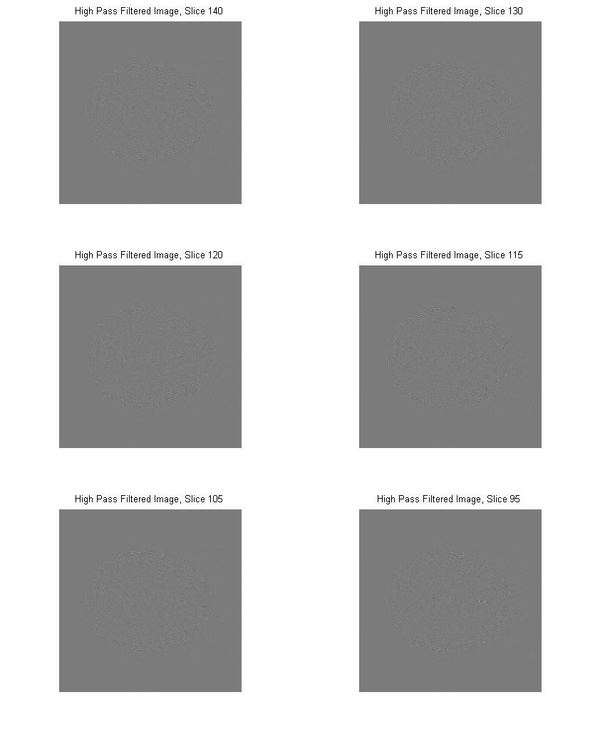
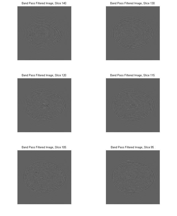
4. In order to account for noise that would occur due to different acquisition times, a Low Pass Filter (LPF), Band Pass Filter (BPF) and High Pass Filter (HPF) were examined. In order to factor in a low pass filter, a threshold at 0.25〖voxels〗^(-1) was taken, thus passing information contained under 0.25〖voxels〗^(-1). The band pass filter passed any information contained in 0.25〖voxels〗^(-1) to 0.75〖voxels〗^(-1). The High pass filter passed any information contained above 0.75〖voxels〗^(-1). Each filter was implemented finding where | 4. In order to account for noise that would occur due to different acquisition times, a Low Pass Filter (LPF), Band Pass Filter (BPF) and High Pass Filter (HPF) were examined. In order to factor in a low pass filter, a threshold at 0.25〖voxels〗^(-1) was taken, thus passing information contained under 0.25〖voxels〗^(-1). The band pass filter passed any information contained in 0.25〖voxels〗^(-1) to 0.75〖voxels〗^(-1). The High pass filter passed any information contained above 0.75〖voxels〗^(-1). Each filter was implemented by finding the indices of each image where the threshold values occurred, then creating a matrix where any values outside the threshold indices are zero. This matrix was multiplied by each Fourier transform of the image to perform the actual filter. | ||
5. In order to test the algorithm matching closely to real life situations, a shift test and noise test was performed. | 5. In order to test the algorithm matching closely to real life situations, a shift test and noise test was performed. | ||
i. In order to perform the shift test, MatLAB functions such as ‘circshift’ were used. The circshift function essentially loops the values from one side of the image to the other. The side of the image with the looped | i. In order to perform the shift test, MatLAB functions such as ‘circshift’ were used. The circshift function essentially loops the values from one side of the image to the other. The side of the image with the looped values was then set to zero for only the amount of indices the image was shifted. Thus, the side that in real life would be shifted off the image was replaced with zeros in order to mimic a real life shift. This shifted image was tested against the non-shifted version of the image. | ||
ii. The second test was to add noise to a file. In order to add noise, the function ‘awgn’ was used in MatLAB. The function would add noise to a file given a certain SNR. In order to test the cross-correlation method, one | ii. The second test was to add noise to a file. In order to add noise, the function ‘awgn’ was used in MatLAB. The function would add noise to a file given a certain SNR. In order to test the cross-correlation method, one image had noise added to it, and it was tested against the same image without noise. | ||
6. Lastly, | 6. Lastly, a median filter was implemented to sift out the undesirable noise. The median filter was found at **add citation** and implemented into the code. | ||
==Theory / Explanation== | ==Theory / Explanation== | ||
Revision as of 07:30, 21 March 2013
Back to Psych 221 Projects 2013
Neuroimaging
Introduction
With the opening of Stanford's Center for Cognitive and Neurobiological Imaging (CNI), we now have access to a large number of MR scans of the human brain. The CNI is closely connected to MR hardware and image processing algorithms used in the cognitive and neurobiological sciences. As a shared facility that is dedicated to research and teaching, the CNI provides resources for researchers and students. The MR images that were used for this project were obtained courtesy of the CNI.
Motivation behind the project
Brain vs Squash Detection

In the field of medicine, students practice taking effective MR scans on inanimate objects such as a squash or pumpkins. In addition, researchers developing MR technology often test new techniques on objects. However, these phantom MR images often get stored into the database of actual human MR images. Sometimes the scans are labelled incorrectly, causing the contents to differ from the label and be a misleading piece of data. This proves to be a major problem and must be rectified without manually going through all the scans. Therefore, the main motivation behind the project was to separate the scans of squash from those of brains so that there would not be trivial errors while maintaining MR databases.

Brain vs Brain Detection
As new brains are added to existing databases, detection of MR scans taken of the same person is desirable in order to prevent duplication. In addition, efficient and accurate matching of brain MRIs may have various medical and research applications.
Project Aim
Thus, the project was divided into two parts:
a) Brain vs. Squash detection
b) Brain vs. Brain detection
Brain vs. Squash detection
The goal of this part of the project is to determine whether a magnetic resonance scan is a brain or squash. Using striking features characteristic to each type of object, files are identified as either brain or squash images. Upon making this distinction, the squash files can be discarded and further work can be carried out on the brain scan.
Brain vs Brain matching
Identify when two MR images are of the same brain (brainprint), even if they were had different contrasts.
Dataset
Sample MR Scans
The MR scans were stored as NIFTI files. The MATLAB code available in the "Tools for NIfTI and ANALYZE images" package was used to load and initially view the MR scans. An example of a brain and a squash file is shown below. [1]
- Brain & Squash: Views
-
 Top, Side, and Front View: Brain MRI
 -
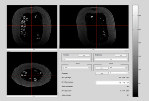 Top, Side, and Front View: Squash MRI


Algorithms
Brain Vs Squash Algorithm

Overview
1. Select a slice from the MR image/scan
2. Perform edge detection on it. Two edges will be obtained
3. Pick short edge
a) Perform Seed Detection
i. Short Edges
ii. Fill Holes
iii. Remove Small Objects
iv. Count Pixels
v. Decide by looking at the threshold.
4. Pick long edge
a) Perform Thickness Determination
i. Calculate thickness
ii. Determine by looking at threshold
5. Combine the results from step 4 and 5.
Explanation
• 1. A file from the database of NIFTI files were selected in MATLAB and this data was scaled as an image and stored in a 3D array. 2D slice images (from approximately 60% up the image in the z direction) were used. 2. Edge detection on the images from the MRI was then performed. In order to execute edge detection, the built-in MATLAB edge detection functions ‘edge’ was used. The edges detection is two types of edges, long and short. 3. Since seeds were present in squashes, but not brains, they were used as one distinguishing factor. To obtain the seeds, the short edges needed to be identified.
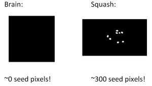
 a) Perform Seed Detection
     i. In order to find seeds, short edge detection was performed on both files.
     ii. For any short edge that was connected as a circle, those areas within the short edges were filled with white pixels to increase the total intensity of the files that have seeds.
     iii. Small, non-seed like objects were then removed.
     iv. All that remains in the image will be seeds, or bits of noise that go through the algorithm.  In order to distinguish between the brain and squash file, the total number of pixels was measured.  This is due to the fact that the seed pixels will be filled in, and everything else will be not.
     v. Since the files with seeds have numerous pixel values, and the files without seeds do not, a threshold is set on the total number of pixels to determine which files obtain the filled in seeds.  The files that give a number above the threshold are determined as seeds
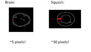
• 4. The other criteria to determine a squash from a brain is the measurement of the outer edges. Since a brain scan has the skull involved also, there are three distinct lines, one being the outer shell of the skull, one being the inner shell, and one being the outline of the brain. The squash on the other hand only has two long edges, and these are separated by an amount that is greater than the separation between the edges of the skull.
 a) Perform Thickness Determination
     i. The distance between the outer edges of both files is then determined.
     ii. A threshold is then set on the number of pixels that is needed between the two long edges.  If the number of pixels between the long edges is high, it is most likely a squash.  If the number of pixels is low, it is most likely a brain.
5. To complete the algorithm, steps 4 and 5 are integrated to give two criteria in determining if a file is a brain or a squash.
Brain / Brain Matching Algorithm
Overview
3D Cross Correlation:
1. Take file.
2. 3D- Fourier Transform
3. Cross-correlation
i. Slide and multiply to determine similarity
3. Normalized: Robust to brightness differences! to the max intensity of each file
4. LP, HP, BP filters
5. Tests
i. Apply shifts to images
ii. Apply noise to images
6. Check Threshold
>90% similarity = MRIs of the same brain
Explanation
The main deterministic factor in the brain matching algorithm is the cross correlation. The files are three dimensional vectors; hence a three dimensional cross correlation is needed. But certain steps are taken to try and ensure a meaningful cross correlation is taken: 1. First two or more files must be selected from the NIFTI database given. 2. In order to calculate the cross correlation the Fourier transform of each file is needed. Using functions such as ‘fftn’ and ‘fftshift,’ the Fourier transform of each file is taken. 3. Cross-correlation
i. The maximum value of the cross-correlation is simply multiplying the Fourier transform of one file by the conjugate of the Fourier transform of the second file and then determining the maximum value. This then returns a non-normalized single value that is characteristic of how well the maximum value their image alike.
3. In order to normalize the cross-correlation, the product of the sum of the all the pixel intensities was taken. Then each maximum value from the cross-correlation was divided by the product of the sum of the vectors. This allows for the maximum value of the cross-correlation of an image with itself to be one. 4. In order to account for noise that would occur due to different acquisition times, a Low Pass Filter (LPF), Band Pass Filter (BPF) and High Pass Filter (HPF) were examined. In order to factor in a low pass filter, a threshold at 0.25〖voxels〗^(-1) was taken, thus passing information contained under 0.25〖voxels〗^(-1). The band pass filter passed any information contained in 0.25〖voxels〗^(-1) to 0.75〖voxels〗^(-1). The High pass filter passed any information contained above 0.75〖voxels〗^(-1). Each filter was implemented by finding the indices of each image where the threshold values occurred, then creating a matrix where any values outside the threshold indices are zero. This matrix was multiplied by each Fourier transform of the image to perform the actual filter. 5. In order to test the algorithm matching closely to real life situations, a shift test and noise test was performed.
i. In order to perform the shift test, MatLAB functions such as ‘circshift’ were used.  The circshift function essentially loops the values from one side of the image to the other.  The side of the image with the looped values was then set to zero for only the amount of indices the image was shifted.  Thus, the side that in real life would be shifted off the image was replaced with zeros in order to mimic a real life shift.  This shifted image was tested against the non-shifted version of the image.
 ii. The second test was to add noise to a file.  In order to add noise, the function ‘awgn’ was used in MatLAB.  The function would add noise to a file given a certain SNR.  In order to test the cross-correlation method, one image had noise added to it, and it was tested against the same image without noise.
6. Lastly, a median filter was implemented to sift out the undesirable noise. The median filter was found at **add citation** and implemented into the code.
Theory / Explanation
Theory Behind Brain and Squash Distinguishing
Two techniques based on detecting two key features were employed to differentiate a brain from a squash image. Firstly, the skull has thin outer layers whilst the phantoms (squash) have a thick outer layer. In addition, the squash have seeds. Edge detection was used to separate these two striking features from the rest of the contents of the brain or squash.
Edge Detection
The basic theory behind the edge detection is based on identifying the points in a digital image at which the image brightness changes sharply or, more formally, has discontinuities. These points are organized into a set of curved line segments termed edges. Since there are innate discontinuities in the MR image intensity at any change in the material properties, edge detection seems to be a good method for identifying seeds in the squash or the layers of the skull or squash. By applying an edge detector to a MRI slice, a binary image containing the set of connected curves indicating the boundaries of objects inside the scan is obtained. Hence, the application of an edge detection algorithm significantly reduces the amount of data to be processed, preserving the the important structures that are being used and filtering out information that is less relevant. This aids in efficient identification of the scan as a brain or a squash. The subsequent task would be to interpret the information contents in the original image, which is substantially simplified.
As edges in images are areas with strong intensity contrasts, the jump in intensity from one pixel to the next is exploited to our advantage. Although edge detection techniques like Prewitt, Sobel and Laplace, the Canny edge detection algorithm seems to be the optimal edge detector. The theory behind Canny edge detection can be broken down into some simple steps:
STEP 1: FILTERING.
The image is processed such that it filters out any noise in the original image. It is essential that image pre-processing is performed before trying to locate and detect any edges.
STEP 2: FINDING EDGE STRENGTH
Next, find the edge strength by taking the gradient of the image. The Sobel operator performs a 2-D spatial gradient measurement on an image. Then, the approximate absolute gradient magnitude (edge strength) at each point can be found. The Sobel operator uses a pair of 3x3 convolution masks, one estimating the gradient in the x-direction (columns) and the other estimating the gradient in the y-direction (rows). The gradient is approximated as |G| = |Gx| + |Gy|
STEP 3: FINDING EDGE DIRECTION
Once the gradient in the x and y directions are known, the edge direction can be determined. Whenever the gradient in the x direction is equal to zero, the edge direction has to be equal to 90 degrees or 0 degrees, depending on what the value of the gradient in the y-direction is equal to. If GY has a value of zero, the edge direction will equal 0 degrees. Otherwise the edge direction will equal 90 degrees. The formula for finding the edge direction is just: theta = invtan (Gy / Gx)
STEP 4: COMPARING EDGE DIRECTION
Once the edge direction is known, the next step is to relate the edge direction to a direction that can be traced in an image. So now the edge orientation has to be resolved into one of these four directions depending on which direction it is closest to.
STEP 5: HYSTERESIS
Finally, hysteresis is performed to eliminating streaking. Streaking is when the edge contour breaks due do the operator output fluctuating above and below the threshold. Once we have computed a measure of edge strength (typically the gradient magnitude), the next stage is to apply a threshold, to decide whether edges are present or not at an image point
Theory Behind Brain - Brain Matching
Cross-correlation
In signal processing, cross-correlation is a measure of similarity of two waveforms as a function of a translation applied to one of them. This is also known as a sliding dot product or sliding inner-product.
Using 3DFFT for analysis was concurred to be the best way to perform image analysis as it is computationally efficient and circular. Subsequently, we divide by square root of the product of the image energies to obtain the values of the coefficients.
Technique used: magnitude of the peak of cross-correlation was used for distinguishing two brain files.
Testing the Brain vs Brain Match Algorithm
Given the fact that multiple MR scans of the same brain were not available for the purpose of this project, the MR scans have been tampered with in two ways so as to create a 'different' brain scan from the original, such that those two scans can be compared and we can distinguish clearly between the two 'different' brain scans from the same brain.
The brain scans were tampered with in the following two ways:
I] Shifting the image:
a) Circular Shift
b) Linear Shift
II] Adding noise to the image
Shifting The Image
The MR image was first shifted and.. **elaborate
Adding Noise to the Image
Image-noise is the random change in brightness or color information in images. It is usually an aspect of electronic noise. It can be produced by the sensor and circuitry of a scanner or digital camera. Image noise can also originate in film grain and in the unavoidable shot noise of an ideal photon detector. Image noise is an undesirable by-product of image capture that adds spurious and extraneous information. Given the fact that multiple MR scans for the same brain we not available for the purpose of this project, the MR scans have been tempered with in two ways so as to create a 'different' brain.
For the purpose of the testing, an image was created adding gaussian noise just so that it could be differentiated from the original image. The noise added was Additive White Gaussian Noise (AWGN). AWGN is a channel model where the white noise is added with a constant spectral density. That is, the white noise has a flat or constant power spectral density. Hence, while Gaussian noise is a type of statistical noise wherein the amplitude of the noise has a Gaussian distribution, whereas Additive White Gaussian Noise is a linear combination of a Gaussian noise and a white noise. Different levels of Signal-to-Noise-Ratio were chosen at random. The images with the added noise look as follows :

After the noise had been added to image for the purpose of testing, the technique of median filtering was employed to filter out the noise. Median filtering is a smoothing technique, where the noise is removed for optimizing the image. It is essential that we preserve the edges. However, at the same time while reducing the noise in the image, it is still essential that we preserve the edges as well. The trade-off is slight, though it still exists. The edges are of critical importance for the visual appearance of images. It has been proved that median filtering is an adequate technique for filtering out small to moderate levels of Gaussian noise as the median filter is demonstrably better than Gaussian blur at removing noise whilst preserving edges for a given, fixed window size. This is image pre-processing where the image is significantly improved as a consequence.
**elaborate elaborate elaborate elaborate
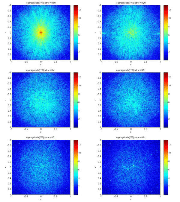
LPF, BPF, HPF for images details.
Low Pass Filtering: A low-pass filter, also called a "blurring" or "smoothing" filter, averages out rapid changes in intensity.
High Pass Filtering:
Band Pass Filtering:
>> mention cut off frequencies we used.
>> all info in lower & nothing/less in higher
>> lower cut off -+0.25, higer -+0.7422
>> briefly talk about ringing
- Low Pass Filter and High Pass Filter Simulated Animations
-
-


- Band Pass Filter and Magnitude Plot (FFT) Animations
-
-


Results
- Brain-Squash Results
-
 Simulated results
 -
 Results of long edges


The normalized cross-correlation maximum was the metric used to quantify the similarity between MRIs. This similarity between twelve randomly chosen brain MR scans are shown in the table below. This data illustrates that the values between two distinct files fall below the similarity metric threshold of 0.9 while the values of the same files are 1 (as expected due to the normalization). Therefore, this is a reasonable choice of threshold.

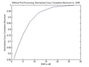
The results from adding white Gaussian noise to a randomly chosen brain MRI and comparing two different noise-added versions of the same scan are shown in the next figure. The noisy images simulate two different acquisitions of the same brain. The normalized cross-correlation maximums are plotted against the SNR of the added noise. The left plot shows the results of the cross-correlation algorithm with no pre-processing of the MRIs while the right plot shows the results from median filtering prior to cross correlation. This illustrates that, using the filtered algorithm, the images are identified as coming from the same brain as long as the SNR is above approximately 7 (the similarity metric falls above the threshold of 0.9), a significant improvement over the unfiltered algorithm.
- SNR results
-
 Normalized Cross Correlation Maximum vs. SNR (Without Pre-Processing)
 -
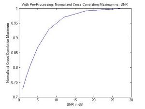 Normalized Cross Correlation Maximum vs. SNR (With Pre-Processing)


This code linearly shifts a randomly chosen brain MRI and compares the shifted and unshifted versions of the same scan using the filtered cross-correlation algorithm. This simulates comparing two acquisitions of the same brain. It plots the normalized cross-correlation maximum against the SNR of the added noise. This illustrates the translation-invariance of the normalized cross-correlation maximum as long as the image does not get cut off. In addition, the images are identified as coming from the same brain (the similarity metric falls above the threshold of 0.9) as long as the shift is less than approximately 95 pixels (for approximately 256x256x256 images).
- Normalized Cross Correlation Maximum vs Shift
-
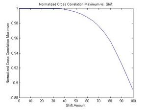 Normalized Cross Correlation Maximum vs Shift


As one can notice the few cross correlation values which stand out are those that are compared with the same file. This happens after adding noise to the band-pass filtered image and then taking a median filter. It means that the algorithm works in distinguishing similar brains. Even though every peak value is not equal to one, they are significantly higher in value than those cross-correlated with different brain images. This indicates the algorithm is able to filter out noise, which simulates different acquisitions of the same brain, and then able to distinguish the similar brains.
As one can see, when the median filter is taken out certain files are falsely determined as similar. This is due to the noise added to the files to simulate different acquisitions. Even though the algorithm does a fairly good job matching similar brains with noise, it is not good enough. Most of the values of different brain values are significantly lower than those matched with the same brain, but due to the false positives, it can skew the data.
As one can see the peak values are those corresponding to comparison with the same brain. These peak values are significantly higher than those compared with different brains. This shows that the cross correlation method without added noise works with integration of the band pass filter.
Conclusions
Initial Struggles
Brain vs Squash Metric
The initial algorithms were about taking slices of the brain near the eyes or the teeth. After obtaining this slice, comparing the eyes or the teeth features with that of the squash and hence differentiate between the two. However, taking a slice near the eyes or the teeth in 3D was a challenge and that it was not an efficient method of distinguishing as even though the eyes and the teeth were striking features, they were not entirely ideal for identification.
Brain vs Brain metric
The initial plan was to record the outer shape of the two brain MR images. If these recorded shapes were similar, then an overlap the two MR images would be done and subsequent difference in the images would be calculated that would then be an indicator of the similarity or the mismatch of the MR images. However, this logic was flawed as it failed to take image contrast, brightness and pixel offsets into consideration. And hence, while taking the difference of the images, even the slightest of pixel offsets would push back the results by a significant amount. Thus, this technique had to be abandoned.
What worked
Brain vs Squash
The fact that slices were taken and worked upon in the 2D domain, rather than the 3D domain helped in solving the brain vs squash detection algorithm. The algorithms employed were based on the fact that a human skull has two layers, narrowly separated and that every squash has seeds; as this is true universally, the detection was successful.
Brain vs Brain
The fact that the 3D Fourier transforms
Future Scope
1] There is much more to be worked on once two brains have been identified to be similar. The areas of working on the process of evaluating the image quality seems to be a promising. The process of taking an MRI scan require patients to hold still for extended periods of time. This ranges from in length from 20 minutes to 90 minutes or more. Thus, considering the fact that the MRI scans can be affected by movement, it is often noticed that problems such as mouth tumors cannot be suitably investigated as the process of coughing or swallowing can make the images that are produced less clear. An interesting prospect would be one where the MRI scan is checked to see if it's been affected by any such kind of movement. And if an error is detected owing to movement, then that MRI scan can be deemed as a flawed one without the need to manually check it. Image registration is the process of transforming different sets of data into one coordinate system. Registration is necessary in order to be able to compare or integrate the data obtained from different measurements. This, in addition to the fact that while images are being processed, factors like noise and inaccuracies would be an interesting prospect to work on.
2] While passing the image through the bandpass filter in the project, there are ringing artifacts that appear as spurious signals near sharp transitions in a signal. These occur because of the usage of a filter with a sharp cut-off frequency. Implementing filters with a smoother cut-off frequency would be something that should be worked on.
3] As humans often have medical procedures performed on them in the course of their lifetime, they often have metallic objects such as dental crowns, dental implants and metallic orthodontic appliances surgically inserted in them. These foreign objects cause artifacts and are a common problem in head and neck MRIs. Work in the field of identifying the metal dental objects that produce artifacts on brain MRIs seems to be a potential area to work on.
4] In recent times, a process called “skull stripping” has been employed on the MR scans. This process involves removal of the scalp, skull and dura, and is an important procedure in brain image analysis. In the event that skull stripping has been performed on an MR image, then one of the metrics used in this project to identify the brain, where we check the width of the two layers of the brain will fail. Thus, in the event that skull stripping has been performed on the image, an interesting future scope for this project would be to shift focus to purely the brain matter with all the tissues, and work on differentiating it's features such as corpus callosum etcetera, from that of the squash. Image segmentation by setting appropriate threshold would be a suggested technique to follow. The removal of dura-matter while leaving brain tissue untouched is especially important when estimating cortical thickness, and could be potentially worked on. [2]
5] In the rare event that the MR scan has been rotated whilst storing, it will prove to be a problem as the project does not deal with the case where the MR scan is a rotated image. Hence, dealing with MR scan rotation and making the algorithm fool-proof seems to be an ideal technique to work one.
References
Papers and Online Material
[1] http://www.mathworks.com/matlabcentral/fileexchange/8797
[2] http://www.lni.hc.unicamp.br/fabricio/papers/2009_Costa.pdf
[3] http://brain.oxfordjournals.org/content/130/5/1432.full.pdf
[4] http://ieeexplore.ieee.org/stamp/stamp.jsp?arnumber=06098259
[5] http://noodle.med.yale.edu/~wang/Research/cviu03_wang.pdf *further study
Software
MATLAB [R2013a (Version 8.1)]
Jasc Animation Shop
Appendix I
Source code, Sample Files, and Figures
Neuroimaging: File:Neuroimaging.zip
Folders Contained:
•Sample NII Files and NIFTI Code
•Brain Matching Code and Results Figures
•Fourier Transform and Filtering Code and Images
•Squash Brain Differentiation Code
•Future Scope Code - Rotation and Scaling
Neuroimaging: File:BrainMatching.zip
Appendix II
Work breakdown
Aparna Bhat
Literature search of brain matching algorithms
Research on theory behind algorithms
Idea for using thickness for brain vs. squash algorithm
Research on theory for future scope of the project
Wiki:
• First draft (layout and writing of several sections)
• HTML code
• Creation of animated figures
MATLAB code:
• Selection of random files
• Automatic file selection without user involvement
• Helped with shifting images and creating a table of cross-correlation values
Anjali Datta
MATLAB: Neuroimaging.zip
• Downloading, opening, and viewing *.nii files
• Brain vs. squash algorithm
• Visualization of Fourier transforms: labeling, scaling, and plotting (using imagesc)
• Low-pass, band-pass, and high-pass filtering of MRIs
• Cross correlation algorithm
• Pre-processing (using medfilt3 function) before cross correlation
• Generation of data and figures: cross-correlation vs. SNR, cross-correlation vs. shift, and cross-correlation table
Literature search on cross correlation algorithms
Research on NIFTI format
Idea of seed detection
Idea of cross-correlation
Exploration of cross-correlation algorithm robust to rotation and scaling
Editing of Wiki
Andrew Zabel
MATLAB: BrainMatching.zip
• 3D Fourier transforms (using fftn function) and plotting (using mesh)
• Addition of noise to images (using awgn function)
• Helped with shifting images and creating a table of cross-correlation values
• Various graphs and plots
Idea for using 3D Fourier transforms
Exploration of additional filtering before cross-correlation (integrating band-pass filter and cross-correlation codes)
Editing of Wiki
Acknowledgements
Help and advice from:
• Professor Brian A. Wandell
• Professor Joyce Farrell
• Professor Robert Dougherty, Research Director Stanford Center for Neurobiological Imaging.
• Henryk Blasinski, Teaching Assistant.