BellMoonVassiliev

Back to Psych 221 Projects 2013

Background and Motivation

Most digital image sensors rely on a color filter array (CFA) in order to sense color, so demosaicing is an important and near-universal part of the imaging pipeline. Demosiacing is by nature error-prone, since it is an attempt to fill in missing data points with educated guesses. However, if there are multiple images of the same scene - whether captured as individual still frames or from a video - then color information which was lost in one image may be captured in another. By performing joint demosaicing on a set of images, we are able to more accurately reconstruct the color of the scene than with a single image.

A second research area within image processing involves combining a series of images of the same scene in order to achieve a higher signal-to-noise ratio (SNR), higher resolution, or both. Work on super-resolution has focused primarily on grayscale data, since RGB data adds several challenges. In particular, the image channels must remain aligned through any filtering operations, or else the colors may be distorted and leave unpleasant fringes. When these multi-image operations are performed after demosaicing, errors from the demosaicing process are treated as "signal" in the following steps. While denoising is often done on raw Bayer images, super-resolution cannot easily done before demosaicing. In this project, we treat demosaicing, super-resolution, and noise reduction as different aspects of the same problem, which is to use all of the information in the source images to produce a single result which most accurately represents the scene as it would have been captured by an ideal camera.

Even though modern image sensors have large pixel count (8MP and up), superresolution remains relevant. It enhances images obtained with digital zoom and adds another dimension of design flexibility: sensor resolution versus computation. Thanks to Moore's law, the energy price of computation is low and continues to fall, but the cost of moving data on and off a chip remains nearly constant constant. Using a sensor with fewer pixels (requiring less data movement) in combination with super resolution techniques may result in a more energy efficient system at the expense of small reduction of image quality. This argument is even stronger for computer vision systems where photographic quality is usually less important.

Our long term project is to create a new programmable ISP chip suited for various computational photography algorithms. With that in mind, goal of the the project was not to find the algorithm with best possible results, but rather an algorithm which can be efficiently implemented in hardware.

Method

Our approach consists of an image alignment step, which finds the relative horizontal and vertical offsets between the LR images, and a demosaicing step which combines the data from LR images into a single HR image. The quality of the reconstruction depends on the camera's sensor and optics, and on the relative alignment of the images.

The combination of the sensor and optics determines the optical point spread function, which in turn determines how difficult it is to obtain a sharp image result. Using multiple images does not reduce or remove the blur induced by the optics; it only provides a higher SNR image.

When multiple images are aligned and averaged, the result is as if the image were convolved with a PSF the size of a pixel. For hypothetical pixels with 100% fill factor, this PSF is a square of exactly the pixel size. Conversely, for pixels with 0% fill factor (i.e, sample points with no area), the PSF is a delta function - and no additional blur is induced. The obvious downside is that a 0% fill-factor pixel cannot capture any light.

In both of these cases, non-blind deconvolution can be applied to the image to sharpen it. However, deconvolution is a complex problem and we did not attempt it in this project. Any resolution improvement we obtain is by reconstructing aliased high frequencies, based on the fact that the sensor fill factor is less than 100%.

The relative positions of the LR images are also important to the reconstruction. In the ideal case, four images are spaced exactly one pixel apart, giving red and blue color samples at every point, and two green samples for every point. In the worst case, the images overlap perfectly, which allows us to average pixels together to reduce the SNR, but does not offer any additional color information. A burst of images from a real camera will generally fall somewhere between these two extremes. As long as the image registration returns the correct offsets, a larger number of images always has the potential for a better result, at the expense of additional computation time.

In this project, we assume ideal camera optics. This is the approach taken by most recent super-resolution and demosaicing works. TODO: cite

Image Alignment

To align the images, we use phase correlation directly on the mosiaced data. To do this we take the Fourier transform of images x and y to get their frequency domain representations, X and Y. The phase correlation P is calculated as

$P={ℱ}^{-1}\left(\frac{X{Y}^{*}}{|X{Y}^{*}|}\right)$

Some works low-pass filter the data in order to mask the effect of the Bayer pattern [6], but we did not find this to be necessary. If the image does not have any strong content, then high frequency induced by the alternating pixel colors will dominate the actual frequencies in the image, and always force a "zero" registration. We found that this was a problem for spatial cross-correlation, but not for phase correlation. Because phase correlation works in the frequency domain, it assumes that the image is circular (i.e, it is continuous from one edge back around to the opposite edge). Since the image is not circular in reality, it can be multiplied by a window function to reduce edge-induced artifacts. However, in our testing, windowing the images did not produce a more accurate registration.

Parabola fit to find subpixel offset. Although the parabola itself is not an accurate fit to the data points over this window, the peak closely matches the actual registration center.

The result of the correlation is a matrix of correlation values, which for a good registration form a single sharp peak. To obtain a subpixel-resolution offset, we fit a parabola to a 7x7 window around the peak, and then solve for the maximum of the parabola. We found that the (rather large) 7x7 window gave more accurate results than 5x5 or 3x3 windows.

We perform correlation between every unique pair of images, which gives us 1+2+...+(n-1) relative offsets. We fix the first image at (0, 0), and then find the image positions which best fit the measured offsets using a least-squares fit. Although our method only measures X and Y translations, it is straightforward to extend the process to handle rotation and scale between images by representing the images with polar coordinates [6].

Hardware considerations - Spatial cross-correlation

Performing large Fourier transforms in hardware is very expensive, since large portions of the image must be in memory at one time. If the pixel offset is very small, then calculating the offset using correlation in the spatial domain may be more efficient than in the frequency domain. Using a number of small patches or a multi-scale optical flow algorithm might allow for a much more efficient hardware implementation for image registration.

If we just look at the asymptotic behavior, correlation in frequency domain is $O(N*log(N))$ operation per each FFT transformation versus $N^2$ for the spacial domain. But in the frequency domain image is replicated, which will produce false results if we choose small patches for calculations. Correlation in the spacial domain does not have this property and thus can use smaller patches.

It's impossible to say exactly what is the boundary when frequency domain is better, because the patch size reduction for spacial domain depends on the data. Find the minimal patch size for both methods is a good research question by itself. However to mitigate the problem of "bad" region selection (like a piece of blue sky for example), multiple patches from different places can be used. Like in RANSAC, each patch votes for an offset and then we use number of votes to pick the result.

To make this even more robust, those patches can be picked form random places in the image instead of some fixed location.

Superresolution

Once all of the images are aligned, we can combine them to form a single higher resolution image. Because the images are typically not offset by a multiple of the 2-pixel Bayer pattern, the data samples have arbitrary (x,y) locations and no longer conform to any particular mosiac. Thus, the algorithm must be able to handle sample points which do not fall on a grid.

Weighted interpolation function

The first method compiles an array of point samples along with their (x,y) locations, which can be arbitrary floating-point values. A grid is overlaid on these samples, with the resolution of the final image. To build the output image, the algorithm works on pixels one at a time:

• The distance from this grid point (i.e, this output pixel) to all of the input pixels is computed
• A Gaussian weighting function is applied based on the distance. The further a sample is from the point in question, the less it contributes.
• The weights are normalized to sum to 1
• The inner product of the weights and the pixel values is taken, and this value is stored as the pixel intensity

This algorithm ensures that the nearest point contributes the most, but that other nearby points are also used. If one point is nearby and the others are far away, the near point's contribution is weighted very heavily, but if two points are equidistant, they will be averaged.

Because the area over which pixels are averaged is actually rather small (${\sigma }^2\approx 1$), the majority of pixels contribute nothing to the output for any given grid point. Rather than using the entire image, it would be vastly more efficient to use only a small neighborhood. However, because the input samples are not on a regular grid, a clever data structure is needed to enable fast access to the neighboring points.

• Super resolution using Gaussian weight function
• 
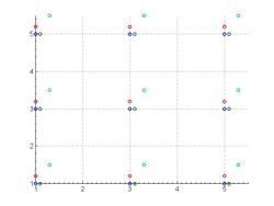  Aligned low resolution images. Each circle color represents samples from a different image.
• 
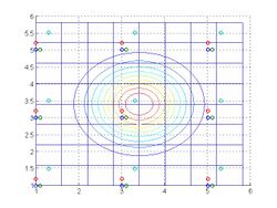  2X resolution grid overlay, with the weighting function for a pixel in the middle. The LR grid is shown with a dashed line; the 2X grid is solid.
• 
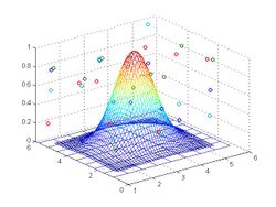  Weight function and data points in 3D

Area averaging

An alternative method we explored treats each pixel as a square, and assumes that LR image registration is only accurate to the first digit after the decimal point. Every data point is replicated 100 times to cover 10x10 area on an intermediate grid. Then we combine all the images at every point by simple averaging followed by an interpolation to fill in the missing data. After that we subsample intermediate values using the final HR grid to get the final result.

• Super resolution using area averaging
• 
  Start with the aligned LR images
• 
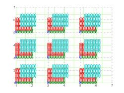  Replicate data samples to the 100x grid
• 
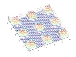  Number of samples per point
• 
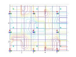  Average and interpolated data at every point
• 
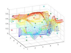  Interpolated data in 3D
• 
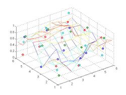  Result after subsampling using desired HR grid

Mapping very pixel value to 10x10 area on the intermediate grid assumes 100% fill factor, but we can easily adjust it to a more realistic model by using rectangles with area close to the real fill factor for a sensor.

Comparison of the interpolation methods

Both methods using averaged existing data to estimate values on the grid.

In our final code we use the weighted Gaussian function because it calculates the missing value in a single step and can be easily extended to perform more advanced demosaicing. However, it requires floating point operations to calculate the weight function and floating point division to normalize the result. By contrast, the area averaging approach requires more intermediate memory and two steps (map to 100x grid with averaging and interpolation), but can use all integer math and no complicated division. For this reason, it is better suited for a hardware implementation. Unlike the MATLAB implementation which allocates memory for the full 100x image array, a hardware implementation would work with a sliding window and thus require far less memory at a single time.

Demosaicking

Principles from single-image demosaicing

Since single-image demosacing is a well-studied problem, we began by implementing a simple demosiacing algorithm.

Before directly working with multiple images for demosaicing, we first apply our demosaicing algorithms to a single image to figure out how effective it is within a single-image framework. Through this experiment, we expected to get some ideas of how to extend this algorithms to multiple-frame demosaicing.

Our algorithm is executed in two steps.

1. Interpolate Green channel by using gradient information of Red and Blue channels.

2. Interpolate Red and Blue by using inter-color correlation parameters, Red-to-Green and Blue-to-Green ratio.

Green Interpolation

Blue Interpolation

Since red and blue channels are down-sampled two times more than the green channel, it's reasonable to interpolate the green channel first then red and blue channel with the interpolated green channel. The simplest approach would be to estimate the unknown pixel values by simple linear interpolation. However, this approach will ignore important information about the correlation between color channels and will cause severe color artifacts. Another critical drawback of simple linear interpolation is that uncorrelated pixels across edges will be averaged and will result in blurred edges. Considering this fact, our algorithm uses second derivatives of the red and blue channel to give different weights for the horizontal and vertical interpolation of the green channel.

Weights are computed from the red or blue channel as follows.

Here is the equation for the second derivatives.

(The formula above is described for the green value estimation at blue points. The unknown values for the green channel at red points can be estimated by the same formular with replacing the blue channel gradients with red channel gradients.)

The intuition behind this algorithm is that second gradients in the blue or red channels imply possible existence of an edge so that we could use different weight for the horizontal and vertical direction interpolation in the green channel. The large value of second gradients implies existence of an edge while the small value implies either uniform color region or uniformly varying color region. Considering this fact, it's reasonable to giver larger weight to the direction with smaller gradient and smaller weight to the direction with larger gradient when interpolating unknown green pixels. This method will help prevent blurring across edges. If both gradients in the horizontal and vertical directions are zero, equal weights are used (0.5) to equally interpolate in both directions.

Now that the unknown pixels in the green channel have been interpolated, inter-color correlation could be taken into account for the unknown pixels in the blue and red channels. Here, we assume that there are correlation between the green and the blue (red) component. This assumption makes sense, because the green spectral power density overlaps with the blue and red spectral power density. After this point, the interpolation process will be explained based on the blue channel interpolation, but the same process is applied to the red channel interpolation.

The blue (red) channel interpolation involves the following two steps.

2-1 Filling in the unknown blue (red) values at the pixels on the green bayer pattern.

These pixels have adjacent known blue (red) values so that those values could be used to interpolate the pixel point. Also, the green value at the pixel point could be used to predict the blue (red) value at the point. The following equations take these two aspects into consideration.

The first term is an average of two neighboring blue values, and the second term uses the green value and the blue-to-green ratio to predict the blue value at the current pixel point. The blue-to-green ratio at the current point can be estimated from the blue-to-green ratio at the adjacent points. (If the adjacent blue values are located vertically, the first term of the equation should take two vertical values instead of horizontal ones)

The weight to the inter-color correlation term (the second term) varies across different images, and we got the following numbers through our own experiment on several test images.

2-2 Filling in the unknown blue (red) values at the pixels on the red (blue) bayer pattern.

At these locations, there are no adjacent blue values. While more intelligent algorithms could be applied to interpolate these pixels, we simply apply linear interpolation with the four adjacent blue values that have been interpolated in the previous phase.

Experimental Results

We compare the result of our demosaicing algorithm with the one that the decmosaic function in Matlab produces.

Test images

We use PSNR and S-CIELAB as the image quality metrics. The results shows that our algorithm usually gives better S-CIELAB number, and this motivates extending this algorithm to the multi-image demosaicing frame work.

File:Test images result.png

Matlab code for the single-image demosaicing

demosaic_single.m - Given a reference image, this function creates RGB bayer pattern out of it, apply our algorithm and Matlab demosaic separately to them, and give PSNR, S-CIELAB values.

test_demosaic_single.m - This script call demosaic_single function with five different test images to extract PSNR and S-CIELAB values.

getPSNR - compute PSNR given a reference image and demosaiced image.

getscielab - comput S-CIELAB value given a reference image and demosaiced image.

Generalization to multiple images

When multiple images with arbitrary translations are merged together, the resulting mesh of sample points no longer forms a Bayer pattern. If rotation and scale are also considered, the mesh is not even regular. Thus, we need to generalize the demosiacing methods to handle an arbitrary configuration of sample points. The Gaussian weighted average described above is able to handle arbitrary sample points, but applied to a single image, it operates effectively the same as bilinear interpolation. Because it does not take cross-channel correlations into account, it discards useful information and tends to produce "zippering" artifacts at sharp edges.

As described above, the solution for single images is to use cues from other channels. If the second derivative of the blue channel is high in the vertical dimension, then interpolating the green values above and below is likely to give a bad result, and these should be ignored. If the second derivative is zero, then interpolating along the vertical direction is likely to give a good result.

Rather than try to perform a curve fit for the data at each upsampled grid point to find the derivative, we do one superresolution pass on the image and then take differences between pixels, which is fast and simple. To determine the vertical-horizontal bias to use, we compute a factor $\alpha$ using the function

$\alpha =\frac{{\partial }^{2}x+k}{{\partial }^{2}x+{\partial }^{2}y+2k}$

where $k$ is a regularization constant. The concept of "red-row pixels" and "blue-row pixels" no longer applies, so we use the sum of red and blue together for $\partial x$ and $\partial y$. To control the direction of interpolation, we adjust the standard deviation of the Gaussian function:

$w=\exp (-(\Delta y^2\cdot 4(1-\alpha )+\Delta x^2\cdot 4\alpha ))$

where $\Delta x$ and $\Delta y$ are the X and Y distances from the interpolation point to the sample point.

Results

We tested our algorithms with synthetic images (e.g, a zoneplate) and with downsampled photographs. We create subpixel offsets by taking weighted averages of neighboring pixels and then downsampling by two. The mosaic pixels are then pulled out of the RGB image and combined into a single mosaiced image. Noise is added to the image, and we then pass the result to our algorithm.

Demosiacing

In these samples, we do not use a higher resolution; we simply perform demosiacing with multiple images.

Truth image

Demosaicing a single image with linear interpolation. Note the strong red/blue artifacts.

Demosaicing with four randomly placed images. The artifacts are reduced, but still present.

Demosaicing with four optimally placed images. Since we now have a color sample for each channel and pixel, no artifacts are present.

Superresolution

In this test, we combine four randomly-shifted images into an image with double resolution, and check against the double-resolution original. In the graph below, we compare the SNR of our result against the result from upsampling a single demosaiced image. Our result has an improved SNR on both synthetic ("zoneplate") and real ("structure") images.

Signal-to-noise ratio comparison of our demosaicing/superresolution method against upsampled images demosaiced with nearest-neighbor, bilinear interpolation, and MATLAB's demosaicing operator.

Steered interpolation

Truth image

Alpha value

There are zippering artifacts in the green channel after weighted Gaussian interpolation

After steering the Gaussian, the zippering artifacts are reduced.

Images with parallax

There is no good way to handle parallax or scene motion where parts of one frame are not visible in another and vice-versa. Not only is it impossible to find a global registration between the images, it is impossible to find a corresponding match for every pixel in an image. It would be possible to use a number of computer vision methods to segment the image and demosaic parts separately, but such algorithms typically do not have the precision necessary for our demosiacing to run well. A more effective way to handle parallax is to eliminate or reduce it it from the outset by capturing the scene at a very high frame rate, perhaps more than 1000 frames per second. At such speeds, the pixel-wise offsets between frames will be in the single digits, and so the global registration assumption is correct, or nearly correct.

Conclusions

Here is where you say what your results mean.

References

[1] S. Farsiu, D. M. Robinson, M. Elad, and P. Milanfar, "Dynamic demosaicing and color superresolution of video sequences", in Proceedings of SPIE, vol. 5562, 2004, pp. 169-178.

[2] S. Farsiu, M. Elad, and P. Milanfar, "Multiframe demosaicing and super-resolution of color images", Image Processing, IEEE Transactions on, vol. 15, no. 1, pp. 141-159, 2006.

[3] M. Guizar-Sicairos, S. T. Thurman, and J. R. Fienup, "Effcient subpixel image registration algorithms", Optics letters, vol. 33, no. 2, pp. 156-158, 2008.

[4] T. Q. Pham, L. J. Van Vliet, and K. Schutte, "Robust fusion of irregularly sampled data using adaptive normalized convolution", EURASIP Journal on Advances in Signal Processing, vol. 2006, 2006.

[5] H. Takeda, S. Farsiu, and P. Milanfar, "Kernel regression for image processing and reconstruction", Image Processing, IEEE Transactions on, vol. 16, no. 2, pp. 349-366, 2007.

[6] P. Vandewalle, K. Krichane, D. Alleysson, and S. Süsstrunk, "Joint demosaicing and super-resolution imaging from a set of unregistered aliased images", in Electronic Imaging 2007. International Society for Optics and Photonics, 2007, pp. 65 020A-65 020A.

Appendix I - Code and Data

All of our code is written in MATLAB and is available on GitHub: [1]

Test data files are also included in the git repository.

Appendix II - Work partition

Artem developed the "area averaging" image merging algorithm, spacial correlation as alternative to FFT and brought hardware implementation considerations. Steven developed the image registration algorithm, the "weighted average" image merging algorithm, and literature references. Donguk implemented and tested the single-image demosaicing algorithm, wrote the error metric scripts and found most of the test images. All three of us collaborated on this wiki page.