WooLee

Back to Psych 221 Projects 2013

Background

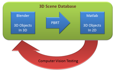
It is no wonder that vision is one of the most important parts in our lives. Besides, due to the tremendous improvements in technology, research on 3D vision has become hot topic. 3D reconstruction is interesting in a way that we could realize a 3D image by just looking at a 2D image. In this project, we provide some techniques for developing scene models that could be used in analysis in ISET. We build the scene using Blender and export it to PBRT files. Then, in Matlab, we run the ISET to analyze the scene converted. We also attempted to do 3D reconstruction, demonstrating a possible way of using scenes for computer vision testing.

Figure 1 Overview

Figure 2

Once you upload the images, they look like this. Note that you can control many features of the images, like whether to show a thumbnail, and the display resolution.

Figure 3

Blender

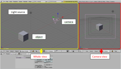
Blender allows us to design 3D objects in 3D space. It has various features, such as modeling, texturing, lighting, animation and video post-processing functionality. Also, it is highly compatible with other files so that we can make use of other 3D files to edit them. The figure below shows basic Blender interfaces.

Figure 2

Take a cube as an example as shown fig.x. There is an object, which is a cube in this example, light source, and camera. On the left side of the figure.x, it shows whole scene that we created, on the right side, it shows the scene which is viewed through the camera. We can control the parameters and the properties of those; - object : edit geometry, size of the object, control reflectance such as diffuse, specular - light source : set light source as you would like to use such as D65 - camera : viewing position, choose lens

In our project, Blender is used for creating scene. There are few steps to do this. 1) import the file Import the file which is filename.dae. 2) texturing

To make texture on the object, texture image is needed, and it should be converted to .tga format. Then we put the texture image on the object. Also, we can apply the material to the object using texture menu shown in the figure. [[File:

3) control reflectance We are able to control reflectance, light source as well. In the case of reflectance, it is allowed to apply diffuse and specular reflectance on the object. [[File:

4) export to pbrt

Finally, the scene has been created by exporting the image to pbrt using exporter. Go to render menu, and click the export to pbrt.

Here are some examples of 3D objects created via Blender. [[File:

Methods

Measuring retinotopic maps

Retinotopic maps were obtained in 5 subjects using Population Receptive Field mapping methods Dumoulin and Wandell (2008). These data were collected for another research project in the Wandell lab. We re-analyzed the data for this project, as described below.

Subjects

Subjects were 5 healthy volunteers.

MR acquisition

Data were obtained on a GE scanner. Et cetera.

MR Analysis

The MR data was analyzed using mrVista software tools.

Pre-processing

All data were slice-time corrected, motion corrected, and repeated scans were averaged together to create a single average scan for each subject. Et cetera.

PRF model fits

PRF models were fit with a 2-gaussian model.

MNI space

After a pRF model was solved for each subject, the model was trasnformed into MNI template space. This was done by first aligning the high resolution t1-weighted anatomical scan from each subject to an MNI template. Since the pRF model was coregistered to the t1-anatomical scan, the same alignment matrix could then be applied to the pRF model.
Once each pRF model was aligned to MNI space, 4 model parameters - x, y, sigma, and r^2 - were averaged across each of the 6 subjects in each voxel.

Et cetera.

Results - What you found

Retinotopic models in native space

Some text. Some analysis. Some figures.

Retinotopic models in individual subjects transformed into MNI space

Some text. Some analysis. Some figures.

Retinotopic models in group-averaged data on the MNI template brain

Some text. Some analysis. Some figures. Maybe some equations.

Equations

If you want to use equations, you can use the same formats that are use on wikipedia.
See wikimedia help on formulas for help.
This example of equation use is copied and pasted from wikipedia's article on the DFT.

The sequence of N complex numbers x₀, ..., x_N−1 is transformed into the sequence of N complex numbers X₀, ..., X_N−1 by the DFT according to the formula:

$X_{k}=\sum _{n=0}^{N-1}x_{n}e^{-{\frac {2\pi i}{N}}kn}\quad \quad k=0,\dots ,N-1$

where i is the imaginary unit and $e^{\frac {2\pi i}{N}}$ is a primitive N'th root of unity. (This expression can also be written in terms of a DFT matrix; when scaled appropriately it becomes a unitary matrix and the X_k can thus be viewed as coefficients of x in an orthonormal basis.)

The transform is sometimes denoted by the symbol ${\mathcal {F}}$, as in $\mathbf {X} ={\mathcal {F}}\left\{\mathbf {x} \right\}$ or ${\mathcal {F}}\left(\mathbf {x} \right)$ or ${\mathcal {F}}\mathbf {x}$.

The inverse discrete Fourier transform (IDFT) is given by

$x_{n}={\frac {1}{N}}\sum _{k=0}^{N-1}X_{k}e^{{\frac {2\pi i}{N}}kn}\quad \quad n=0,\dots ,N-1.$

Retinotopic models in group-averaged data projected back into native space

Some text. Some analysis. Some figures.

Conclusions

Here is where you say what your results mean.

References - Resources and related work

References

Software

Appendix I - Code and Data

Code

File:CodeFile.zip

Data

zip file with my data

Appendix II - Work partition (if a group project)

Brian and Bob gave the lectures. Jon mucked around on the wiki.