Hsu

Back to Psych 221 Projects 2013

Introduction

The proliferation and wide availability of digital cameras has made detection tampering a prominent topic, especially in legal or political situations. Detection based on color filter array (CFA) interpolation seeks to use frequency patterns introduced by demosaicking to detect tampering of an image. Popescu and Farid analyze the frequency patterns of a probability map to detect tampering [1] while Dirik and Memon analyze artifacts of demosaicking to detect image tampering [2]. This project is based off of algorithms used in [1].

Background

While images files are usually represented in three color channels, digital cameras typically only have one image sensor. For the sensor to capture three different light wavelengths, a color filter array (CFA) is placed in front of the image sensor so that each pixel is only allowed to capture a narrow spectrum of light. The most common type of CFA is the Bayer filter (shown in the figure on the right), which is divided between red, green, and blue light. The Bayer filter uses 50% green pixels since the human eye is more sensitive to green light. This work assumes that all test images employ the Bayer filter.

Bayer filter array. (www.analog.com)

CFA Interpolation

After the image is captured by the sensor, the channels are interpolated into a full three-channel color image. This section will describe basic linear interpolation techniques.

Linear and Single Channel

The simplest form of CFA interpolation interpolates each color channel separately using linear filters. Examples of linear filters include:

1. Bilinear: Biinear filters interpolate by taking the linear average of neighboring pixels. For the green channel, this is represented as ${\begin{bmatrix}0&{\frac {1}{4}}&0\\{\frac {1}{4}}&0&{\frac {1}{4}}\\0&{\frac {1}{4}}&0\end{bmatrix}}$ where each interpolated pixel is the average of its neighboring pixels
2. Bicubic: Bicubic filters require an 8x8 filter and calculates the weighted average of 16 pixels. For the green channel, the bicubic matrix is ${\begin{bmatrix}0&0&0&1&0&0&0\\0&0&-9&0&-9&0&0\\0&-9&0&81&0&-9&0\\1&0&81&256&81&0&1\\0&-9&0&81&0&-9&0\\0&0&-9&0&-9&0&0\\0&0&0&1&0&0&0\end{bmatrix}}$ where each interpolated is the average of its neighboring pixels

Gradient

A gradient-based CFA interpolator keeps edge information by conditioning the interpolation direction on gradients in all directions and involves all three color channels in each color channel interpolation. The gradients between red and blue pixels is first calculated in all directions and the lowest directions of gradients are selected as the direction the pixels will be averaged in. This keeps pixels from smearing across sharp transitions. The red and blue channels are computed by averaging the difference between the red/blue channels and the green channel.

Smooth Hue

A smooth hue filter averages hue to interpolate images. Hue is the ratio between the red/blue channels and the green channel, and missing pixels are bilinearly interpolated according to hue.

The section above shows that CFA interpolation can introduce regular patterns into interpolated image since the interpolation filter results in dependence between the pixels. These regular patterns can be used to detect tampering of an image because the frequency spectrum of the interpolated pixels will be changed if a section of the image is altered. This project assumes that the Bayer filter is used and that the interpolation used is linear.

Methods

The expectation-maximization algorithm from [1] calculates an estimation of the linear model used to interpolate the Bayer array and generates the per-pixel probability that each sample pixel belongs to the calculated linear interpolation filter. The probability map was then analyzed for periodic frequencies to detect image tampering.

Expectation-Maximization Algorithm

Expectation

The expectation step of the algorithm estimates the per-pixel probability that the pixel belongs to the estimated linear model, α. Each color channel is described as

$f(x,y)=\sum _{u,v=-N}^{N}\alpha _{u,v}f(x+u,y+v)+n(x,y)$

where $n(x,y)=f(x,y)-\sum _{u,v=-N}^{N}\alpha _{u,v}f(x+u,y+v)$ is the residual error between the actual image and the estimated image. The residual error is approximated using a Gaussian function with zero mean and $\alpha$ standard deviation. The probability that each pixel is taken from the estimated linear model is calculated using the probability distribution function of the residual errors:

$P(x,y)={\frac {1}{\sigma {\sqrt {2\pi }}}}exp\left[-{\frac {1}{2\sigma ^{2}}}\left(f(x,y)-\sum _{u,v=-N}^{N}\alpha _{u,v}f(x+u,y+v)\right)^{2}\right]$

Using this probability, the per-pixel probability that the image is estimated by the proposed $\alpha$ is calculated using Bayes' rule. In these calculations, only the proposed linear model and an unspecified non-linear model were considered as possibilities. The non-linear model M_{2} was estimated to be one over 255;

Failed to parse (Conversion error. Server ("https://wikimedia.org/api/rest_") reported: "Cannot get mml. TeX parse error: Undefined control sequence \emph"): {\displaystyle \Pr\{{\emph {f(x,y)}}\in M_{1}\mid {\emph {f(x,y)}}\}={\frac {\Pr\{{\emph {f(x,y)}}\mid {\emph {f(x,y)}}\in M_{1}\}\Pr\{{\emph {f(x,y)}}\in M_{1}\}}{\sum _{i=1}^{2}{\Pr\{{\emph {f(x,y)}}\mid {\emph {f(x,y)}}\in M_{i}\}\Pr\{{\emph {f(x,y)}}\in M_{i}\}}}}}

Maximization

The maximization step of the algorithm computes a revised α based on minimization of the residual error. The error function that is minimized is:

$E(\alpha _{newu,newv})=\sum _{x,y}w(x,y)\left(f(x,y)-\sum _{u,v=-N}^{N}\alpha _{u,v}f(x+u,y+v)\right)^{2}$

Minimization of the residual error is calculated by setting the partial derivative of the error function with respect to each element of α to zero. The resulting system of linear equations can be solved for a new α estimation. The algorithm stops when the difference between subsequent α arrays is sufficiently low.

Tamper Detection

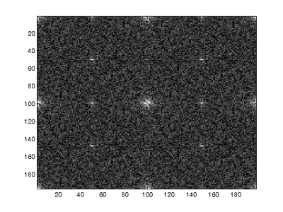
Since the probability maps generated by the E-M exhibit regular frequencies corresponding to the CFA interpolation patterns, the FFT of the probability maps for untampered images will show identifiable frequency peaks. This occurs because the E-M algorithm will assign high probabilities to interpolated pixels since the interpolated pixels roughly follow a linear model. The pixels that represent data collected by the camera will exhibit low probabilities since the linear approximation of the pixel will result in larger error. The images below show the FFTs of probability maps over untampered and tampered regions of an image.

Measure of Similarity

Tamper detection was implemented by calculating the similarity between an ideal probability map and the estimated probability map. The similarity function is given by:

$M(p,s)=\sum \limits _{w_{x},w_{y}}{P\times S}$

where P is the Fourier transform of the calculated probability map and S is the Fourier transform of the ideal probability map for each channel. The similarity between the ideal and calculated probability maps determines whether or not the image has been modified; high similarity indicates that the given CFA interpolation of the image can be approximated using a linear array since the frequency content of the probability map will be close to ideal. In contrast, tampering changes the frequency content of the probability map and the frequencies between the ideal and real case will result in a lower similarity measure.

Ideal FFT of green channel.

P was not normalized since the algorithm compares the frequency content between blocks of the image. Normalization would introduce localized scaling factors, which would vary between blocks.

Windowing

Given that the tampered areas in the training images were small areas of the main image, a sliding window was used to calculate the measure of similarity for segmented blocks of the image. This prevented the slight spatial frequency differences in the probability map caused by tampering to be overshadowed by the much larger regular frequency in the non-tampered parts of the image. The windows with the smallest measure of similarity are identified as tampered regions and server to localize the tampered region.

Threshold

Ideally, a minimum threshold for the measure of similarity can be determined to automatically detect tampered regions. Windows that have a measure of similarity below a certain threshold would be considered tampered images. Unfortunately, the threshold was difficult to determine due to:

1. Variation in frequency content between windows
2. Variation in frequency content between images
3. Low frequency content of uniform color patches in images

In particular, the low frequency content of uniform color patches, such as walls or the sky, was difficult to solve since the frequency spectrum of uniform patches is very similar to that of tampered images. In these cases, the probability maps are uniform since adjacent pixels show the same value, which corresponds to DC frequency content. Tampered images also show high DC frequency content since the tampered regions do not show a regular periodic pattern. The results section will discuss the efficacy of alternatives to detection based on frequency spectrum.

Since the measure of similarity was not normalized, the mean and standard deviation was calculated for each image and the threshold (in standard deviations) determined based on the training set of images.

Results

Threshold Detection

Measure of Similarity

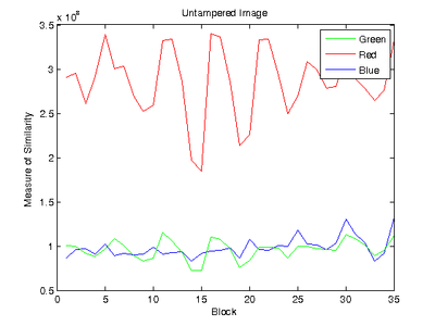
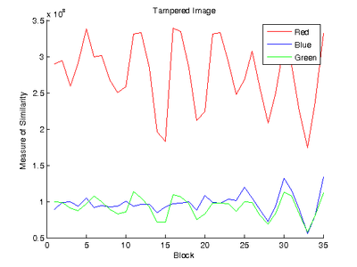
The measure of similarity result showed high block-to-block variation, which resulted in difficulty when comparing all blocks in the image. As shown in the figures below, there is high variation between blocks as well as a central spike at Block 15 that corresponds to a section of blurred soil in the photo. In addition, while the effect of tampering is clearly seen at Blocks 27 and 33, the signal strength of the tampered blocks is very close to that of Block 15. This shows that the signal distribution of blurry and uniform sections in the photograph creates opportunities for false positives when applying automatic tamper detection. The effect of uniform sections in the photograph can be mitigated by larger block sizes at the expense of looser tamper localization constraints.

Number of Iterations

Given the difficulty in differentiating between tampered regions and uniform color regions, additional metrics were tested to determine whether or not the regions could be separated. First, the number of iterations of the E-M algorithm was recorded to find if tampered regions required more iterations to converge to a small error value. The figure below shows the number of iterations per block required where the tampered region straddles Blocks 7 and 8. While the number of iterations increases in Block 7, the number of iterations decreases in Block 8, which indicates that iterations is not a consistent metric for differentiating between tampered regions and uniform regions.

Conclusions

An algorithm was implemented to determine the periodic information of three-channel color images as a method to detect digital tampering. A simple linear model was assumed for the images although more complex models should yield better results. Automation was a key difficulty in this project because not every image had consistent thresholds. In addition, uniform regions within the image had frequency spectrums similar to regions that were tampered.

Future Work

Future work that could yield better results include using more complex models across different color channels. In addition, a metric is needed to distinguish between areas of uniform color and tampered areas.

References - Resources and related work

The majority of this project were drawn from [1]. Matlab was used to implement the algorithms.

[1] A.C. Popescu and H. Farid. Exposing Digital Forgeries in Color Filter Array Interpolated Images. IEEE Transactions on Signal Processing, 53(10):3948-3959, 2005.

[2] Dirik, A.E.; Memon, N., "Image tamper detection based on demosaicing artifacts," Image Processing (ICIP), 2009 16th IEEE International Conference on , vol., no., pp.1497,1500, 7-10 Nov. 2009.

Appendix I - Code and Data

Code

File:CodeFile.zip

Data

Images used for testing were provided by the class.