Stephanie Pancoast, Aaron Zarraga, Edouard Yin

Introduction

In order to obtain a high quality image from a digital camera sensor, it is necessary to demosaick color filter array (CFA) values to estimate RGB values for each pixel. It is also important to apply a denoising algorithm to make the image look crisp and clean. Challenges arise, however, when trying to match a demosaicking and denoising algorithm. Many demosaicking algorithms are created under the assumption that the CFA values are free of noise:

"...most demosaicking methods are developed under the unrealistic assumption of noise-free data. In the presence of noise, the performances of the algorithms degrade drastically, since their sophisticated nonlinear mechanisms are generally not robust to noise. Moreover, denoising after demosaicking is untractable, because demosaicking distorts the characteristics of the noise in a complex and hardly computable form." - Laurent Condat

For this reason, "denoisaicking" algorithms have been developed to combine denoising and demosaicking. The purpose of this project is to implement, analyze, and characterize one such denoisaicking algorithm written by Laurent Condat. We use a "simple" algorithm (a bilinear demosaick followed by a linear color correction) as a baseline for comparison.

Methods

For this project, all major calculations and algorithms were implemented in Matlab.

Overview of Condat's Algorithm

Note: In order to run Condat's algorithm on a Mac, some of Condat's code may not run correctly. You may need to download special files that have been compiled to run on Macs.

Condat's algorithm essentially builds on the demosaicking technique called "frequency selection". This algorithm estimates the Red/Blue and Green/Magenta chrominance channels by modulating the CFA input and convolving the result with a low pass filter. The estimation of these two channels is then remodulated and subtracted from the original input to estimate the luminance channel values.

Condat creates his denoisaicking algorithm by denoising after two main steps. The algorithm denoises the chrominance channel estimations and then once more after the luminance channel estimation.

Note on Hardware Performance: The convolutions estimating the two chrominance channels are expensive operations. However, they are independent and could be implemented in parallel on a chip.

Pipeline Integration

For our testing, we edited wrapperimage.m to call Condat's algorithm instead of the simple version. In order to integrate Condat's algorithm, we first had to normalize the provided CFA values so they would be in a range that Condat's algorithm expects. Condat's algorithm expects values in the range from 0-255, and the CFA contains values ranging from 0 to ~5. To calculate this normalization, we created a "cfa_factor":

cfa_factor = 255/max(CFA) (where max(CFA) is the maximum value found in the CFA matrix)

We scaled the CFA matrix by multiplying it by cfa_factor. We then fed this normalized CFA into Condat's algorithm. To compensate for this adjustment on the output of Condat's algorithm, we divided the output by cfa_factor. The figure below shows the integration of Condat's algorithm into the wrapperimage pipeline.

After this was complete, we were getting visible images out of the wrapperimage pipeline, but the images were pink. This is due to the fact that Condat's algorithm and the wrapperimage use shifted versions of the Bayer CFA. In order to fix this problem, we removed the first the first column of pixels. (This is acceptable, since the metrics scripts ignore the outer 10 pixels).

Condat's algorithm takes in the CFA as well as a standard deviation estimate for the noise present. To complete the integration of Condat's algorithm into the wrapperimage pipeline, we wanted to experiment with this noise parameter to see if we could improve the performance of the denoisaicking. Instead of using the suggested value of 25 (based on a range of 0-255), we calculated the actual standard deviation of the noise added to the image. In practice, this parameter would be unavailable, but we wanted to push the parameter to its limit. We found that by using the actual standard deviation of noise, we were not able to perform any better than with using the magic "25" estimation. Therefore, we kept this parameter at 25 for the remainder of the project.

Metrics

We obtained metrics for our pipeline by not only examining the metrics calculated in the provided project code, but also by conducting a "preference survey" with over 100 people. This allowed us to evaluate the denoisaicking algorithm both quantitatively and qualitatively. It was interesting to see how well the numerical metrics matched up with people's preferences. This will be discussed in more detail in a later section.

Results

- Eddie

Organize your results in a good logical order (not necessarily historical order). 
Include relevant graphs and/or images. Make sure graph axes are labeled.
Make sure you draw the reader's attention to the key element of the figure.
The key aspect should be the most visible element of the figure or graph.
Help the reader by writing a clear figure caption.

Using the framework built by Steven Lansel, we could test Laurent Condat's joint denoising and demoisaicing algorithm. This framework gives us the possibility to simulate different conditions of luminosity for a given scenery, and to add in some realistic noise. Then we can feed those images to the algorithm in test and get processed images as outputs. Moreover this framework provides us with some metrics on the quality of the output images.

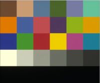
To understand better the qualities and defaults of this algorithm, it is interesting to compare the output images for very different kinds of input images. We tested this algorithm with six different input images, selected for being representative of different kinds of pictures and for the different challenges the pictures can pose. Additionnally, we tested the algorithm on the MacBeth color checker.

Here is an example of the outputs we got from this framework:

We can see that the algorithm gives very good images for high luminosity. From the human point of view, the resulting images seem almost perfect to perfect. However in low luminosity, the quality of the images is not as good: the algorithm was not able to reconstruct all the data from the noisy image.

To have an objective measure of the quality of the output images, we used several metrics: MCC color bias, MCC color noise, delta E in S-CIELAB metric space, and signal-to-noise ratio. We used those metrics to compare our output images to those obtained from using a simple pipeline applying sequentially demoisaicing and denoising.

MCC-color-bias	MCC-color-noise	S-Cielab delta E	SNR

MacBeth Color Checker

Looking at the plots for MCC color bias, we can see that the difference between the algorithms in MCC color bias is neglectable. Using joint denoising and demoisaicing does not reduce further the measured color bias. On the other side, the plots for MCC color noise are very different. Condat's algorithm performs much better than the simple pipeline. This difference is reflected by the absence of grain in our outputs, as opposed to those coming from the simple pipeline. Condat's algorithm output images are smoother and has decreased the noise more efficiently.

MCC for simple pipeline	MCC for Condat's algorithm

S-CIELAB

The S-CIELAB metric is an extension of the CIELAB metric to include the effect of spatial pattern on human vision. We used the S-CIELAB metric to measure the visual difference between the original image and the output image. The plot shows two different domains: - on low luminosity, the joint denoising-demoisaicing performs better than the simple pipeline. - on higher luminosity, it performs not as well as the simple pipeline.

The shift between those domains is at approximately 50 cd/m².

However, at this point, the delta E value is only 4. Considering that human vision accepts differences of delta E of a few units, the human eye would not be disturbed significantly by the error left out by our algorithm.

Here is another example of outputs, for a very different kind of input image:

This image shows how the algorithm behaves on details. The foliage is a very difficult part to handle because of its very high frequency patterns. We can see that the foliage tends to be blurred even, independently of the luminosity.

Conclusions

- Edddie - Describe what you learned. What worked? What didn't? Why? What would you do if you kept working on the project?

Further improvements

If given more time, we wish to improve on Laurent Condat's algorithm. Laurent Condat fixed several coefficients that parameter his denoisaicing. For example, he uses a fixed sigma value of 25. We would like to try different values of sigma and compare the delta E for each one of those values. This would give us a better default value of sigma. Second, we would try having a dynamically value for sigma instead of a sigma value: based on the intensity of the ambient light, we can predict the characteristics of the noise. During this class, we learned that the standard deviation of the noise can be approximated as the value of the square root of the light intensity. Therefore, given the XYZ values of a normally noised picture, it is possible to evaluate the value of sigma, and to feed it to Condat's algorithm.

Besides, if given even more time, we would like to write Condat's algorithm in an actual programming language, such as C. The time measurements would then be more relevant. A further step would be to write this code in Verilog. This would give us the performances of a dedicated chip, that would be embeddable in a camera.

References

1) Laurent Condat's homepage

2) A simple, fast and efficient approach to denoisaicking: joint demosaicking and denoising

Appendix I

Code

Put description of stuff inside zip here... File:Pipeline Code.zip

make clicking on file download it

Survey Results

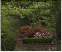
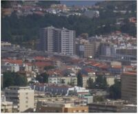
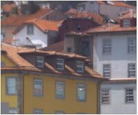
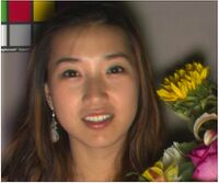
Using SurveyMonkey, we asked for people to choose which of two side by side images they prefer. The results of this survey are summarized below. The questions are listed in the order they appeared along with the corresponding image and luminance value that served as the input for the denoisaicking and simple pipeline. Some responders did not answer every question.

Survey Results

Question	Image #	Lum. (cd/m^2)	Prefer Condat	Prefer Simple
A	2	2	58	42
B	6	6	80	20
C	1	2000	1	99
D	4	200	60	40
E	5	600	15	85
F	3	200	41	55
G	7	3	82	13
H	6	600	11	84
I	3	6	82	13
J	5	2000	11	83
K	7	200	51	35
L	4	2	62	25
M	2	60	67	28
N	1	3	27	59

do I need to discuss the results or is that done in conclusion section?

Images

Luminocity = 6cd/m^2	Luminocity = 600 cd/m^2	Original

• Upload source code, some result images, etc, and give a description of each link.

In some cases, your acquired data may be too large to store practically. In this case, use your judgement (or consult one of us) and only link the most relevant data. Be sure to describe the purpose of your code and to edit the code for clarity. The purpose of placing the code online is to allow others to verify your methods and to learn from your ideas. It should be possible for someone else to generate result images using your code.

Appendix II

All members of the group worked equally on obtaining the code and figuring out how to adapt to the wrapper files provided to us at the beginning of the project. This was the main aspect of the assignment. The remainder was broken down as follows:

Stephanie Pancoast

• Modified provided code to save files and display images
• Created survey and compiled results to test human component of algorithm
• Human component aspect of presentation
• References, Appendix I, and Appendix II sections of Wiki

Edouard Yin

• Tested effectiveness of scaling sigma values according to noise in image
• Modified code to account for magnitude scaling
• Metric results aspect of presentation
• Results and Conclusions sections of Wiki

Aaaron Zarraga

• Modified code to account for magnitude scaling
• Studied Condat's algorithm closely to better understand what the code was doing
• Algorithm aspect of presentation
• Introduction and Methods section of Wiki

Back to Main Page