Matt

VARIATION IN SIGNIFICANT CLUSTER NUMBER AND DISTRIBUTION DUE TO PARAMETER SELECTION DURING CORRECTION FOR MULTIPLE COMPARISONS USING THE MONTE CARLO METHOD IN FUNCTIONAL MAGNETIC RESONANCE IMAGING DATA

Background

When conducting statistical analysis it is important to be aware of the problem of multiple comparisons. The problem of multiple comparisons arises when more than one statistical test is considered simultaneously. When more than one statistical test is conducted, there is an increased likelihood that any single test will reach significance for rejection of the null hypothesis compared to if a single test were ran. Importantly, criterion for null hypothesis rejection can be altered to help accommodate for multiple statistical tests. One example of multiple comparison correction is the Bonferroni method, which requires the single-test p-value rejection threshold to be divided by the number of tests conducted. For datasets in which many statistical tests are necessary to make inferences, methods like the Bonferroni correction may be too severe, resulting in strongly reduce power.

The problem of multiple comparisons often occurs in statistical analysis of brain imaging data, where analysis can often be conducted on data from more than one channel, voxel, dipole source, temporal bin or spatial location. For example, in functional magnetic resonance imaging (fMRI), there are often more than 10,000 voxels from which data is statistically analyzed. If 10,000 signals were created using a random number generator, simply by chance alone many signals would likely appear to be significant, that is, if not corrected for multiple comparisons. Many methods have been developed to deem whether a particular fMRI signal is significant. One such method uses Monte Carlo simulations.

The Monte Carlo method includes four major steps, first a domain needs to be designated (a space for values), second values need to be assigned to the spaces identified in the first step in a random manner, third and lastly, a pre-specified calculation needs to be ran on these values to assess probability of outcomes. The values should be truly random and many. In fMRI applications, Monte Carlo simulations can be used to assess statistical power of a cluster of voxels identified at a given voxel-wise p-threshold. Such a Monte Carlo simulation may use a volume of voxels as the domain, a random number generator for input assignment (n(0,1) per voxel), and a calculation of the size of clusters at given threshold to quantify probabilities of observed outcomes. Such a Monte Carlo simulation can be repeated multiple times to achieve increasingly precise and stabile estimates, and the resulting cluster sizes can be averaged across iterations.

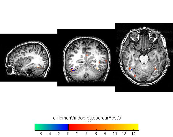
In the current study, I used a previously collected dataset (detailed below) to explore the effects of parameter selection (voxel-wise p-threshold) in Monte Carlo simulation on the characteristics of significant voxel clusters. The variation in cluster size and distribution is subsequently discussed. I hypothesize that at more stringent voxel-wise p-thresholds the clusters will be smaller and more statistically significant on average, per voxel.

Below is another example of a reinotopic map in a different subject.
Figure 2

Once you upload the images, they look like this. Note that you can control many features of the images, like whether to show a thumbnail, and the display resolution.

Figure 3

Methods

Measuring retinotopic maps

Retinotopic maps were obtained in 5 subjects using Population Receptive Field mapping methods Dumoulin and Wandell (2008). These data were collected for another research project in the Wandell lab. We re-analyzed the data for this project, as described below.

Subjects

Subjects were 5 healthy volunteers.

MR acquisition

Data were obtained on a GE scanner. Et cetera.

MR Analysis

The MR data was analyzed using mrVista software tools.

Pre-processing

All data were slice-time corrected, motion corrected, and repeated scans were averaged together to create a single average scan for each subject. Et cetera.

PRF model fits

PRF models were fit with a 2-gaussian model.

MNI space

After a pRF model was solved for each subject, the model was trasnformed into MNI template space. This was done by first aligning the high resolution t1-weighted anatomical scan from each subject to an MNI template. Since the pRF model was coregistered to the t1-anatomical scan, the same alignment matrix could then be applied to the pRF model.
Once each pRF model was aligned to MNI space, 4 model parameters - x, y, sigma, and r^2 - were averaged across each of the 6 subjects in each voxel.

Et cetera.

Results - What you found

Retinotopic models in native space

Some text. Some analysis. Some figures.

Retinotopic models in individual subjects transformed into MNI space

Some text. Some analysis. Some figures.

Retinotopic models in group-averaged data on the MNI template brain

Some text. Some analysis. Some figures. Maybe some equations.

Equations

If you want to use equations, you can use the same formats that are use on wikipedia.
See wikimedia help on formulas for help.
This example of equation use is copied and pasted from wikipedia's article on the DFT.

The sequence of N complex numbers x₀, ..., x_N−1 is transformed into the sequence of N complex numbers X₀, ..., X_N−1 by the DFT according to the formula:

$X_{k}=\sum _{n=0}^{N-1}x_{n}e^{-{\frac {2\pi i}{N}}kn}\quad \quad k=0,\dots ,N-1$

where i is the imaginary unit and $e^{\frac {2\pi i}{N}}$ is a primitive N'th root of unity. (This expression can also be written in terms of a DFT matrix; when scaled appropriately it becomes a unitary matrix and the X_k can thus be viewed as coefficients of x in an orthonormal basis.)

The transform is sometimes denoted by the symbol ${\mathcal {F}}$, as in $\mathbf {X} ={\mathcal {F}}\left\{\mathbf {x} \right\}$ or ${\mathcal {F}}\left(\mathbf {x} \right)$ or ${\mathcal {F}}\mathbf {x}$.

The inverse discrete Fourier transform (IDFT) is given by

$x_{n}={\frac {1}{N}}\sum _{k=0}^{N-1}X_{k}e^{{\frac {2\pi i}{N}}kn}\quad \quad n=0,\dots ,N-1.$

Retinotopic models in group-averaged data projected back into native space

Some text. Some analysis. Some figures.

Conclusions

Here is where you say what your results mean.

References - Resources and related work

References

Software