Eric Burkhart, Eunjoon Cho, James Painter

Introduction

To a user, a digital camera feels straightforward - look at a scene, take a picture, and the image comes out looking like the scene. Inside the case, there's a complex processing pipeline required to transform the raw data into that image. This complexity comes from two limitations in the data - noise and a color filter array (CFA).

The CFA is an array of sensors, one per pixel of the final image, that collects incoming light from the scene. The problem is that each node in the array only outputs a single number instead of one number for every wavelength to which the human eye responds. This causes two problems - first an algorithm needs to estimate the value of red, green, and blue at all pixels, and second each sensor has spectral sensitivities at all wavelengths even though it's value ends up representing a single color. Demosaicing methods have been established to determine the value of missing colors at each pixel using neighboring values.

The sensors themselves are subject to a variety of noises - shot noise, read noise, fixed pattern noise, reset noise, dark current noise, etc. Some of these noise sources can be calibrated out while others cannot be avoided. As a result, denoising methods are an important step in transforming raw data to a high quality image.

For many years, the denoising and demosaicing steps were performed seperately with the first step complicating the noise for the next one. The pipeline explored in this project, implemented using an algorithm by L. Zhang, X. Wu, and D. Zhang, combines these steps to avoid that problem.

Methods

Zhang Paper: Joint Denoising and Demosaicing of Channel Dependent Noise

There are 3 main steps used in the Zhang algorithm.

1. Estimate primary difference signals (PDS)

From the original CFA values the Zhang paper aims to estimate the primary difference signals, $X_{GR}=X_{G}-X_{R},X_{GB}=X_{G}-X_{B}$. The intuition behind this is that natural images are usually pastoral colors and thus these PDS values are more smooth and easier to estimate from noisy measurements. For simplification purposes we assume $X=X_{GR}$ and only consider one of the two PDS. The other can be generalized and measured in the same manner. First, there is a demosaicing step where the missing green and red values are estimated to calculate the PDS. The demosaicing step is a across channel interpolation and it refers to values outside its color channel. We later see that this causes some color bias when the power levels of each channel are different. We compensate for this color offset by introducing a algorithmic modification to take care of this misalignment in color power levels.

From this, we have an estimate of the PDS, ${\bar {X}}_{i}^{d}=X_{i}+\epsilon _{i}^{d}+v_{i}^{d}$, where $\epsilon _{i}^{d},v_{i}^{d}$ is the interpolation error and the sensor noise respectively. We can assume the interpolation error is the error introduced at the across channel interpolation step and is irrelevant to the actual sensor noise that exists at each pixel. The algorithm then applies LMMSE estimates to recover $X_{i}$ and uses first and second moments of the observation and underlying values, i.e., ${\bar {X}},X$.

2. Estimate green channel for all pixels The next step is to have an estimate of the green channel for all pixels based on the de-noised estimate of PDS($X$) in the previous step. The green channel can be estimated from the original noisy CFA values and the de-noised PDS. For example the green value at a noisy red pixel would be as follows.

${\tilde {G}}={\tilde {R}}+X_{GR}=(R+v_{R})+(G-R)=G+v_{R}$

We can see from this equation, the green value estimate at a red estimate reduces to the true green value plus a noise variance at that specific pixel (in this case it happened to be $v_{R}$ since it was in a red pixel). To achieve this estimate of G where the noise distribution is non-stationary across channels, Zhang transfers the variables using wavelet transformations. Then they apply LMMSE on the corresponding wavelet coefficients to achieve an estimate on the underlying value $G$.

3. Estimate remaining channels for all pixels The final step is to recover the other R, B values across all channels. One result we get from the second step is that we have an estimate of the variance across all channels, $v_{C},c\in (R,G,B)$. With this we are able to recover the true R and B values at it's respective pixels. The Zhang paper refers to a previous paper that does demosaicing but mentions that any standard demosacing method will suffice.

Modifications

Implementation

• Shift in the Bayer Pattern: The Bayer pattern provided in the project code was a 90 degree counter-clockwise rotation of that assumed by the default Zhang implementation. To fix this we rotated the CFA pattern in the project code, although shifting the first column of the image by one would have also worked.
• Input Range Scaling: The Zhang implementation requires a 0-255 input value whereas the project provides a 0-1 value. We scaled the values by 255 going into Zhang's denoising/demosaicing step and then scaled back once it output the result.

Algorithmic

• Power level normalization: The Zhang interpolation method incorporates the magnitude of all nearby pixels, not just those of the same color. As a result, a pixel with a high green component would cause nearby red and blue pixels to interpolate to higher than expected values. To fix this we scaled the input values of each channel independently based on the largest entry in that color channel (i.e. redScale = 255/maxRed, greenScale = 255/maxGreen, blueScale = 255/maxBlue). After getting the results from Zhang's denoising/demosaicing step, we the undid that scaling by dividing the result by the scale factor.

Results

Our tests were generated using three images with different amounts of edges. We applied three types of noise to the images' CFAs before passing them through the denoising-demosaicing algorithm: 1. Signal-dependent 2. Channel-dependent, channel-constant, Gaussian (same standard deviation for each channel) 3. Channel-dependent, channel-variable, Gaussian (variable standard deviation for each channel)

Our baseline for comparison is a bilinear interpolation, or "simple pipeline."

All SCIELAB measurements taken were in XYZ space and assumed the image occupies 20 degrees of visual angle.

Introduction to results here! Might be nice to have a table outlining numbers?

Sample Images

Signal-Dependent Noise

Luminance Level (cd/m^2)	60	200	600	2000
Bilinear
Zhang Improved

Luminance Level (cd/m^2)	60	200	600	2000
Bilinear
Zhang Improved

Luminance Level (cd/m^2)	60	200	600	2000
Bilinear
Zhang Improved

Channel-Dependent, Channel-Constant Gaussian Noise

Luminance Level (cd/m^2)	60	200	600	2000
Bilinear
Zhang Improved

Luminance Level (cd/m^2)	60	200	600	2000
Bilinear
Zhang Improved

Luminance Level (cd/m^2)	60	200	600	2000
Bilinear
Zhang Improved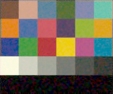

Channel-Dependent, Channel-Variable Gaussian Noise

Luminance Level (cd/m^2)	60	200	600	2000
Bilinear
Zhang Improved

Luminance Level (cd/m^2)	60	200	600	2000
Bilinear
Zhang Improved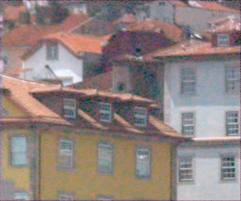

Luminance Level (cd/m^2)	60	200	600	2000
Bilinear
Zhang Improved

Metrics

Signal-Dependent Noise

Channel-Dependent, Channel-Constant Noise

Channel-Dependent, Channel-Variable Noise

Differences From An Ideal Image

We discovered that the Zhang algorithm performs best within smooth regions of the images, and worst at edge regions. This explains the low SNR in the leafy image, which is almost entirely edges, and the high SNR in the other two images, which have many smooth regions. The following delta images illustrate the performance of the algorithm at edges and at smooth regions, for a luminance level of 2000 cd/^2.

Leafy image, original vs. delta

MacBeth image, original vs. delta

The data in the metrics table above also shows that the Zhang algorithm works best with channel-dependent noise, which is the noise distribution that is assumed in the paper.

Zhang vs. "Improved" Zhang

The improvement we made in the Zhang algorithm made a significant difference in all the test images. The difference is clear in images with skin tones, where the decrease in brightness is more apparent after running the original Zhang algorithm. With our improvement, the brightness level is relatively consistent. These images are at 600 cd/m^2 luminance and were given signal-dependent noise.

Face image, original vs. Bilinear

Face image, original vs. Zhang

Face image, original vs. Improved Zhang

Color Accuracy

The following MCC images display the color accuracy of the Zhang Improved (left) and original Zhang (right) pipelines as compared to the original image (middle). By comparing the mean SCIELAB differences on a smooth image with many colors, we get a good picture of the overall color accuracy.

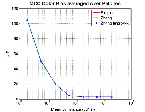
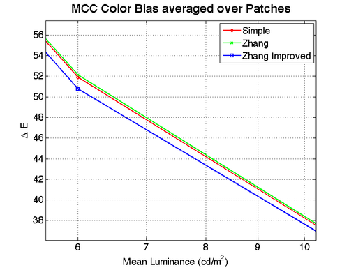
The following graphs show the actual SCIELAB deltaE difference between the images in XYZ space using a 20 degree visual angle for the image. The first shows results at all light levels, and the second is a zoomed in version to display the difference. Since the deltaE difference between Zhang and Zhang improved is near 1 at low luminance and decreases from there as luminance increases, the change in XYZ space is unlikely to be visible. From the images above however in RGB space this difference is more visible.

Noise Elimination: Smooth Regions

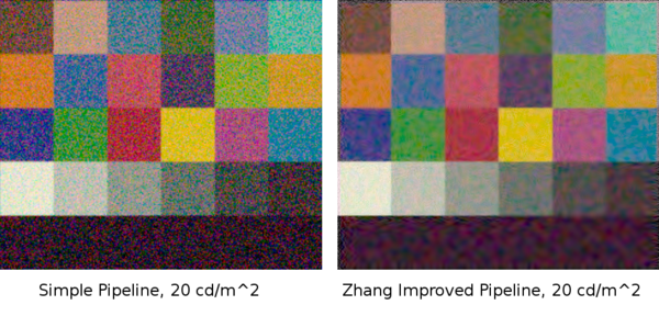
To test noise elimination in smooth regions of an image, we used the image of a Macbeth color checker due to the smooth nature of each color patch. The output of the simple pipeline at 20 cd/m^2 is on the left and the Zhang Improved output for the same image is on the right.

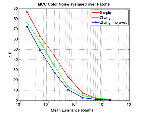
The results over all seven light levels used are shown in the graph below using the SCIELABS delta E metric. The largest improvements come at the low light levels.

Computation Time

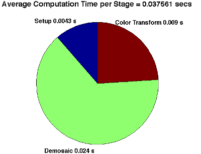
The computation time for the simple pipeline is about 1/40th of a second while the improved Zhang method takes over 15 seconds.

Conclusions

According to SNR and SCIELAB metrics, our modification to the implementation of Zhang's algorithm improves performance in almost all cases (for very low luminance, the unmodified version does better by up to 1 dB in SNR). This modification addresses the problem of color bias by compensating for each color channel having a different power level.

After our modification, Zhang's method outperforms the basic bilinear interpolation demosaicing approach for all three noise models in both the SNR and SCIELAB metrics. The largest performance gains for Zhang's algorithm over the simple pipeline were seen for the noise model addressed in the paper - additive white Gaussian channel dependent noise with differing standard deviations in each color channel.

If we had more time, we would like to take real CFA data from a camera and test the performance of this algorithm. In this project the ISET noise models do not include the channel dependent noise that this algorithm was designed to address. As a result, we used an unrealistic additive white Gaussian noise to display the algorithm's abilities. It would be useful to see how it performs in a real world case where there may actually be different noise standard deviations in each color channel.

In terms of computation time, Zhang's algorithm takes 635 times longer to run than bilinear interpolation. This is about 15 seconds on a standard PC in 2011, meaning the current implementation may be too slow to see practical use. Further work may be able to speed up the algorithm either through more efficient code or hardware acceleration. Also, with the open source camera project [1] the implementation of the pipeline could potentially be moved to a PC in order to make it viable.

Finally, the SNR and SCIELAB metrics are useful for measuring fidelity to the ideal image but that ideal image may not be the most visually appealing representation. We subjectively preferred the output of the unmodified Zhang algorithm to the original image. If the end goal of a pipeline is to sell devices to real people, this is an important point to keep in mind.

References

Papers

L. Zhang, X. Wu, and D. Zhang, "Color Reproduction from Noisy CFA Data of Single Sensor Digital Cameras," IEEE Trans. Image Processing, vol. 16, no. 9, pp. 2184-2197, Sept. 2007. [2]

Software

1. ISET Code [3]
2. Zhang Algorithm Matlab Code [4]

Appendix I - Code and Data

Code

Uploaded with data below

Data

All source files and data needed to run the algorithm

Appendix II - Work partition

Eric Burkhart: Researched improvements to color transform, searched for the color bias problem (thanks Eunjoon for finding it!), partial generation of results, partial writeup
Eunjoon Cho: Integration of Zhang algorithm into pipeline, implemented improved Zhang algorithm to reduce color bias offset, "algorithm" and part "discussions" slides
James Painter: Integration of Zhang algorithm into pipeline, partial generation of result images/metrics, "results" sections of slides and writeup