Medical imaging: Simulations of human oral mucosa tissue fluorescence

Introduction

Autofluorescence spectroscopy has emerged as a promising noninvasive technique since it can diagnose oral neoplasia with sensitivity and specificity [1]. Clinical data indicate that neoplastic progression in the oral cavity is associated with a number of characteristic spectral changes, which come from the altered optical properties of both the superficial epithelium and the underlying stroma [2, 3]. These changes include an increase in epithelial cell scattering, increased stromal hemoglobin content, and decreased structural protein fluorescence within the stroma. Therefore, the interpretation of fluorescence spectra collected in vivo in terms of these biochemical and morphologic changes is crucial. To understand better on how these optical parameters can alter the intensity and shape of the fluorescent spectra, and thereby guide the spectra interpretation to physiological changes, we developed a Monte Carlo model using MCMaltab with site-specific input to simulate the fluorescence spectra on normal, and damaged oral sites. Our goal in developing this model was to provide a computational tool to study how the morphological characteristics of the tissue affect the final fluorescent spectra.

Background

Two key toolings employed to develop our simulation model is EEM and MCMatlab.

EEM

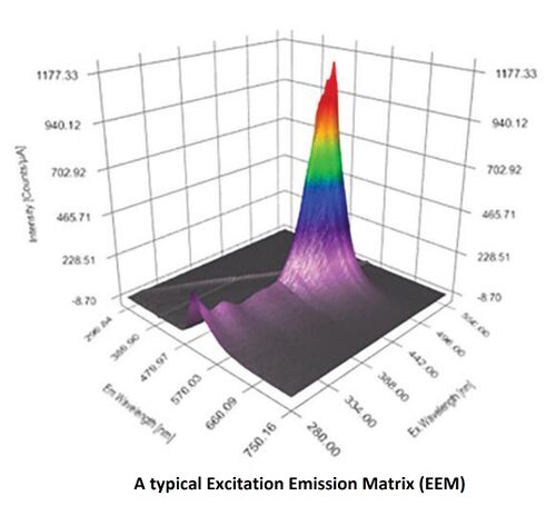
A measurement becoming more widely used in the field of fluorescence spectroscopy is the Excitation Emission Matrix (EEM). An EEM is a 3D scan, resulting in a contour plot of excitation wavelength vs. emission wavelength vs. fluorescence intensity. EEMs are used for a variety of applications where multi-component analysis is required and are often referred to as providing a molecular fingerprint for many different types of samples. EEM is used to well describe the fluorescent property of the fluorophores. Below shows a typical EEM.

MCMatlab

MCmatlab is a Monte Carlo simulation for modeling light propagation in a 3D voxel space [4]. The Radiative Transfer Equation (RTE) is commonly solved with Monte Carlo techniques, starting from modeling the paths of photons traveling through the tissue as a random walk. Monte Carlo simulations statistically sample the step size of the random walk and angular deflection per scattering event, yielding, after averaging over many photons’ paths, realistic approximations to light’s propagation in tissue. It is usually combined with MATLAB to generate the input optical properties of tissue types for a given illumination, allowing the users to create the three-dimensional (3D) structure of the desired heterogeneous tissue. Fluorescence can optionally be simulated after simulation of the excitation light, with 2 additional parameters provided: The fluorescent wavelength and Quantum yield of the fluorophores.

Simulation Model

Our simulation model is developed to account for generation and propagation of fluorescent light in multilayered oral tissue. Tissue fluorescent property is described by EEM from measurement, and then is used as input to the Monte Carlo model to generate predictions of fluorescence spectra. Light propagation in tissue is modeled by MCMatlab.

To be more specific, we simulated the fluorescence of human oral mucosa tissue in oral cavity. In general, for mucosa tissue, the top layer is composed of epithelial cells (called stratified squamous epithelial layer). These cells contain NADH and FAD tissue fluorophores which play an important role in cell metabolism and respiration. The thickness of this layer depends on where in the oral cavity the tissue is, it can vary from 99 ± 22 μm at the floor of the mouth [5], 294 ± 68 μm in the cheek (bucacal mucosa) [5] to 593 ± 63 μm [6]. Underneath the epithelial cells is a basement membrane which is defines a transition from the epithelial cells to the lamina propria where there are collagen fibers and blood vessels. Collagen is another tissue fluorophore (i.e. fluoresces). The lamina starts at a depth of 290 ± 29 μm [6]. The basement membrane is very thin. To simplify the model, we ignore the lamina propria layer, and tissue reflectance, but constructing the tissue model as only one epithelium layer with FAD and NADH fluorophores. When tissue is damaged, Keratin, another fluorophore, will grow on top of the epithelium. So we will conduct simulation focusing on 3 fluorophores: Keratin, FAD and NADH. EEMs from measurement are used to describe fluorescent property. EEM datasets for FAD/NADH/Keratin are obtained from shared database. Light propagation within oral tissues is modeled by MCMatlab. We finally studied the relation of the tissue fluorescence with respect to different excitation wavelength, and the fluorophores at different tissue depths. Our model is validated by matching the simulation results with known knowledge on fluorescent excitation and emission.

Methods

In MCMatlab simulation, we need to determine 2 components of model settings: 1. Geometry model; 2 Media property model; to construct our oral tissue model.

Geometry Model

Geometry model in MCMatlab is used to build a 3D model object with multiple voxels where the light is propagating through, which includes specifying below key inputs:

- Dimensions of the model cuboid: By specifying the side lengths Lx, Ly, Lz.

- Number of bins along each axis of the model cuboid: By specifying the resolutions Nx, Ny and Nz. (Bins denote the granularity at which the volume can be bifurcated into its component media.)

- Positions of each media within the concerned cuboid: By assigning the media index for each voxel in the “GeomFunc” at the end of the model file. The media index is corresponding to the “j” defined in “mediaPropertiesFunc” at the end of the model file. Media definition in “mediaPropertiesFunc” is introduced in Media Property Model.

In our study, as introduced earlier, human oral tissue can be simplified into a 3-layer structure geometry model: Epithelium layer with FAD and NADH beneath; then with/without Keratin layer on top of it. Therefore, 2 configurations: Air-FAD-NADH and Keratin-FAD-NADH are simulated in our study. For the dimension size of the simulation volume, X and Y are set to 300μm. For the thickness of every single layer Z, we all use the site-specific clinical values in practice, which are obtained from Ref. [2]. In prior work, Monte Carlo simulation result is found to be very sensitive to the thickness settings [3]. Therefore, using the practical site-specific tissue thickness rather than the general tissue thickness will make our simulation more accurate. In all, please refer to below table for all the geometric parameters used in our MCMatlab simulation.

Figure 1 present the 3D model geometry illustration of our human oral mucosa tissue constructed in MCMatlab. The top blue layer is either Air or Keratin; the middle orange layer represents the FAD in epithelium layer; and the bottom yellow layer represents the NADH in epithelium layer.

Media Property Model

Once the geometry set up done, media for each voxel needs to be defined in the next step to complete building up the comprehensive model. In MCMatlab, this can be done by modifying or adding to “mediaPropertiesFunc” at the end of the model file. It may optionally include the fluorescence properties as well. To be more specific, each medium can be specified with three optical parameters and one fluorescent property below:

1. μa — Absorption Coefficient in units of 1/cm. May be (a) scalar, (b) a function handle taking wavelength as input or (c) a function handle taking wavelength, FR, T and FD as inputs.
2. μs — Scattering Coefficient in units of 1/cm. May be (a) scalar, (b) a function handle taking wavelength as input or (c) a function handle taking wavelength, FR, T and FD as inputs.
3. g — The scattering anisotropy (the mean cosine to the scattering angle), to be used in the Henyey-Greenstein phase function. It has no units. May be (a) scalar, (b) a function handle taking wavelength as input or (c) a function handle taking wavelength, FR, T and FD as inputs.
4. QY — The quantum yield of fluorescence, that is, photons of fluorescence emitted relative to excitation photons absorbed. It has no units. May be (a) scalar, (b) a function handle taking wavelength as input or (c) a function handle taking wavelength, FR, T and FD as inputs.

In addition, we need to complete two wavelengths setting as well:

1. Set MonteCarlo wavelength to Excitation wavelength;
2. Set Fluorescence MonteCarlo wavelength to Emission wavelength.

In our study, right after 3-layers geometry built up in Geometry Model, we input all optical parameters of these 4 voxels to “mediaPropertiesFunc” for our simulation:

 Air Layer

   μa [cm-1]: μa=1e-8 [7];
   μs [cm-1]: μs=1e-8 [7];
   g: g=1 [7];

μa, μs and g for Air are all constants, and the values are obtained from MCMatlab standard tissue example.

 FAD/NADH/Keratin Layer Layer 

   μa [cm-1]:
   a.	μa=3 (non-fluorescent) [2];
   b.	μa=A/thickness (fluorescent);

The absorption coefficient is considered different for two conditions. When input light wavelength is beyond excitation range, the fluorophore is not excited and not emit fluorescence, μa is considered as constant 3 for simplification. This assumption and value were used in Ref. [2]. Otherwise, we use the formula μa=A/thickness for calculation. A is the absorbance, and we use the excitation matrix from each fluorophore EEM for it in our simulation. Apparently, it is wavelength dependent, and should be more accurate than the constant assumption.

   μs [cm-1]:
   μs_FAD/NADH = 51.9*((523/λ_Excitation)^0.6;
   μs_Keratin = 160.3*((523/λ_Excitation)^0.6;

We use the wavelength dependent scattering coefficient empirical formula μs=μ0*((523/λ)^0.6 [8] to calculate out μs. This formula is from last year's class report and code. Then we use μs = 66 cm-1 at 350nm (λ) in Ref. [2] to calculate out μ0 = 51.9 cm-1 at 523nm for FAD/NADH, and μs = 204 cm-1 at 350nm (λ) for Keratin in Ref. [2] to calculate out μ0 = 160.3 cm-1 at 523nm for Keratin. Then substitute μ0_FAD/NADH and μ0_Keratin back to the empirical formula, so that we obtained μs_FAD/NADH and μs_Keratin expression as above. In some paper, people also assume μs is a constant. But wavelength dependent scattering coefficient empirical is more accurate.

   g: 
   g=0.9 [9].

This value is also obtained from MCMatlab "FluorescenceAndImage" example.

   QY:
   QY= EEM/(1-10^(-A))/2;

We use the fluorescence intensity formula

   ${I_{f}}$=${I_{0}}$*kφ[1-10^(-εbc)] 

to calculate out the quantum yield of the fluorophore, where ${I_{f}}$ is the fluorescence intensity, ${I_{0}}$ is the incident light intensity, k is a proportionality constant attributed to the instrument, ε is the molar absorptivity, b is the path length, and c is the concentration of the substrate. ${I_{f}}$/${I_{0}}$ is EEM for each fluorophore. k=2 in our simulation, verified by normalized fluorescence intensity between 0.1-0.2. φ is the quantum yield; and εbc=A, A is absorbance. We use excitation matrix from each fluorophore EEM to represent A. λ_Excitation, λ_Emission, A, EEM are all extracted from dataset of FAD/NADH/Keratin Excitation Emission Matrixes shared in Database.

Results

We investigated the relation of the tissue fluorescence with respect to different excitation wavelengths. Apparently, the excitation wavelength determined which fluorophore at different tissue depth was excited, and accordingly the final fluorescent emission spectrum and intensity.

Below shows a typical example where FAD, NADH and Keratin layer is excited and fluorescent respectively at the specific excitation wavelength and emission wavelength. For NonKeratin-FAD-NADH 3-layer structure, when the excitation wavelength is 450nm, Fig. 2(d) shows light is mainly absorbed by FAD layer. FAD is excited and provides the fluorescent emission, as shown in Fig. 2(j); while when the excitation wavelength is 340nm, Fig. 2(e) shows light is mainly absorbed by NADH layer. Then NADH is excited and provides the fluorescent emission, as shown in Fig. 2(k). For Keratin-FAD-NADH 3-layer structure, when the excitation wavelength is 285nm, Fig. 2(f) shows light is mainly absorbed by Keratin layer. Therefore, Keratin is excited and provides the fluorescent emission, as shown in Fig. 2(l).

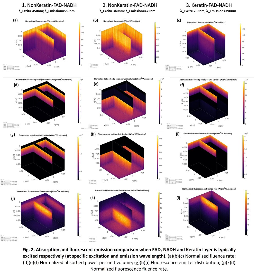
In addition, we plot out the fluorescence emitted light as a function of wavelength, with peak wavelength in the excitation light as a parameter, to investigate which peak excitation wavelength generates the maximum fluorescence. For Air-FAD-NADH 3-layer model, we scanned the input light wavelength from 425nm to 480nm. Absorption and fluorescent emission in Fig. 2(d) and (j) indicate that FAD is mainly excited and fluorescent during these excitation range. Fig. 3 shows the simulation results. It turns out:

1. 460nm generates the maximum fluorescent emission, since it is the best wavelength for FAD excitation.
2. FAD has a peak emission at wavelength of ~550nm.

Our simulation results match with result in other’s work, such as Fig. 4 as attached above [10]. Need to note that slight discrepancy is subjected to EEM of the fluorophores used in the simulation may be different.

For Air-FAD-NADH 3-layer model, we scanned the input light wavelength from 310nm to 390nm. Absorption and fluorescent emission in Fig. 2(e) and (k) indicate that NADH is mainly excited and fluorescent during these excitation range. Fig. 5 shows the simulation results. It turns out:

1. 350nm generates the maximum fluorescent emission, since it is the best wavelength for NADH excitation.
2. NADH has a peak emission at wavelength of ~475nm.

Our simulation results match with result in other’s work, such as Fig. 4. Similarly, different EEM of the fluorophores used in the simulation may result in slight discrepancy.

For Keratin-FAD-NADH 3-layer model, we scanned the input light wavelength from 270nm to 295nm. Absorption and fluorescent emission in Fig. 2(f) and (l) indicate that Keratin is mainly excited and fluorescent here. Fig. 6 shows the simulation results. It turns out:

1. 280nm generates the maximum fluorescent emission, since it is the best wavelength for Keratin excitation.
2. Keratin has a peak emission at wavelength of ~380nm.

Our simulation results match with result in other’s work.

Conclusions

In this study, we developed a model to account for the generation and propagation of fluorescent light in multilayered oral tissue. Clinical site-specific data, including thickness of each oral tissue layer and measured EEM for fluorophores, are used as input to the Monte Carlo model to generate predictions of fluorescence spectra, in order to enhance the accuracy and reliability of the simulation result. We applied this model to simulate oral tissue fluorescence with 3 fluorophores: FAD/NADH/Keratin. Our simulation results match with known knowledge on fluorescent excitation and emission, validating our model. This model can be a very helpful computational tool to study how the morphological characteristics of the tissue affect the final fluorescent spectra. In future, more studies can be done in terms of this model, such as changing the thickness of each single layer, scanning the input wavelength in overlapped excitation range of two or more fluorophores, or adding the lamina propria layer using the EEM for collagen, or adding the blood absorbance, to investigate the impact on the fluorescence.

Reference

[1] C. S. Betz, M. Mehlmann, K. Rick, H. Stepp, G. Grevers, R. Baumgartner, A. Leunig, “Autofluorescence imaging and spectroscopy of normal and malignant mucosa in patients with head and neck cancer”. Lasers Surg. Med 25, 323–334 (1999). [PubMed: 10534749]

[2] I. Pavlova, C. R. Weber, R. A. Schwarz, M. D. Williams, A. M. Gillenwater, and R. Richards-Kortum, “Fluorescence spectroscopy of oral tissue: Monte Carlo modeling with site-specific tissue properties,” J. Biomed. Opt. 14(1), 014009 (2009).

[3] I. Pavlova, C. Redden-Weber, R. A. Schwarz, M. Williams, A. El-Naggar, A. Gillenwater, and R. Richards-Kortum, “Monte Carlo model to describe depth selective fluorescence spectra of epithelial tissue: applications for diagnosis of oral precancer,” J. Biomed. Opt. 13, 064012 (2008)

[4] D. Marti, R. N. Aasbjerg, P. E. Andersen, and A. K. Hansen, “MCmatlab: an open-source, user-friendly, MATLAB-integrated three-dimensional Monte Carlo light transport solver with heat diffusion and tissue damage,” J. Biomed. Opt. 23(12), 1 (2018).

[5] E. Gentile, C. Maio, A. Romano, L. Laino, A. Lucchese. “The potential role of in vivo optical coherence tomography for evaluating oral soft tissue: A systematic review”. J. Oral Pathol. Med. 46, 864– 876 (2017) DOI: 10.1111/jop.12589.

[6] D. Di Stasio, D. Lauritano, F. Loffredo, E. Gentile, F. Della Vella, M. Petruzzi, and A. Lucchese, “Optical coherence tomography imaging of oral mucosa bullous diseases: A preliminary study,” Dentomaxillofacial Radiology 49(2), 20190071 (2020).

[7] “Example1_StandardTissue.m” Example in MCMatlab.

[8] Ritvik Sharma, Pranil Joshi, Arjun Deopujari, “Blood oxygen modelling from skin reflectance” Last year's class report and code.

[9] “Example5_FluorescenceAndImaging.m” Example in MCMatlab.

[10]https://www.becker-hickl.com/faq/can-i-excite-nadh-fad-simultaneously-for-metabolic-imaging/

Appendix

Source Code and EEM Dataset:

https://github.com/wuxuansg/Tissue-Fluorescence-MCMatlab