WenkeZhangChien-YiChang: Difference between revisions
imported>Student221 |
imported>Student221 |
||
| Line 17: | Line 17: | ||
==== Lense Shading ==== | ==== Lense Shading ==== | ||
[[File:cc1.png|thumb|500px|center|An illustration of the lens shading effect.]] | |||
Lens shading, also known as lens vignetting, refers to the phenomenon where the light falls off towards the edges of an image when captured by digital camera systems. Lens shading occurs because in the imaging system with an optical lens, the off-axis pixels often receive a smaller bundle of incident rays compared to on-axis pixels, resulting in relatively lower illumination towards the edges. This effect is ubiquitous and not surprisingly can be observed in the data we collected for the Cornell box lighting estimation. | Lens shading, also known as lens vignetting, refers to the phenomenon where the light falls off towards the edges of an image when captured by digital camera systems. Lens shading occurs because in the imaging system with an optical lens, the off-axis pixels often receive a smaller bundle of incident rays compared to on-axis pixels, resulting in relatively lower illumination towards the edges. This effect is ubiquitous and not surprisingly can be observed in the data we collected for the Cornell box lighting estimation. | ||
| Line 37: | Line 39: | ||
Here the left-hand side is the lens shading matrix and the right-hand side is the normalized image with the lens shading effect. | Here the left-hand side is the lens shading matrix and the right-hand side is the normalized image with the lens shading effect. | ||
In our experiment, we took images of empty background within the Cornell box. We set the lighting condition to be uniformly distributed so that the original image can be approximated as <math>cJ</math>. In order to minimize the random error, images are captured using different exposure duration, ISO speed, and color channels. In particular, we study the red color channel of captured images. This choice is arbitrary and one may find similar results by using different channels. Note that by selecting a single color channel, we essentially downsample the image to half of its original size. After the downsampling, we perform standard averaging and normalization for the single-channel image. We then fit a two-dimension surface to the data using Matlab plugin Curve Fitting. We then upsample the fitted function back to the original dimension using standard interpolation and renormalize the result to obtain the lens shading matrix <math>M</math>. In the code snippet below we show part of our source code that performs the above manipulations. | [[File:cc2.png|thumb|500px|center|An illustration of camera sensor and pixel arrangement.]] | ||
In our experiment, we took images of empty background within the Cornell box. We set the lighting condition to be uniformly distributed so that the original image can be approximated as <math>cJ</math>. In order to minimize the random error, images are captured using different exposure duration, ISO speed, and color channels. In particular, we study the red color channel of captured images. This choice is arbitrary and one may find similar results by using different channels. Note that by selecting a single color channel, we essentially downsample the image to half of its original size. | |||
[[File:cc3.png|thumb|500px|center|By selecting the red channel, we essentially downsample the original image by a factor of two.]] | |||
After the downsampling, we perform standard averaging and normalization for the single-channel image. We then fit a two-dimension surface to the data using Matlab plugin Curve Fitting. We choose a 2D polynomial as shown below: | |||
[[File:cc4.png|thumb|500px|center]] | |||
We then upsample the fitted function back to the original dimension using standard interpolation and renormalize the result to obtain the lens shading matrix <math>M</math>. In the code snippet below we show part of our source code that performs the above manipulations. | |||
%% data preprocessing | %% data preprocessing | ||
| Line 75: | Line 88: | ||
mask = Vq - min(Vq(:)); | mask = Vq - min(Vq(:)); | ||
mask = mask ./ max(mask(:)); | mask = mask ./ max(mask(:)); | ||
== Results == | == Results == | ||
Revision as of 11:41, 6 December 2020
Introduction
Background
Methods
Overview

Light Modeling
Physical Based 3D Scene Rendering
Camera Modeling
Lense Shading

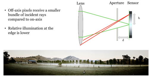
Lens shading, also known as lens vignetting, refers to the phenomenon where the light falls off towards the edges of an image when captured by digital camera systems. Lens shading occurs because in the imaging system with an optical lens, the off-axis pixels often receive a smaller bundle of incident rays compared to on-axis pixels, resulting in relatively lower illumination towards the edges. This effect is ubiquitous and not surprisingly can be observed in the data we collected for the Cornell box lighting estimation.
In this project, our goal is to accurately estimate the lighting condition for the Cornell box. In order to do this, we first need to deconfound the lens shading effect from the empirical data. One way to achieve this is to preprocess the captured images to remove the lens shading effect and then compared the preprocessed images with the simulated ones. Equivalently, we can apply the artificial lens shading effect to simulated images and then compare it with real images. Here we opted for the latter method.
We first assume that the lens shading effect can be represented as element-wise matrix multiplications
,
where is the lens shading matrix, is the original image, and is the image corrected by lens shading effect. We also assume that the lens shading matrix is of the same dimension as the orignal image , and . The problem is equivalent to finding the lens shading matrix . Once we have found the lens shading matrix, we can apply the lens shading effect to any image by simply multiplying it elementwisly against .
In order to estimate the values of the lens shading matrix , let us consider the case where , where is the matrix of ones where every element is equal to one and is a constant. We have
,
and equivalently
.
Here the left-hand side is the lens shading matrix and the right-hand side is the normalized image with the lens shading effect.

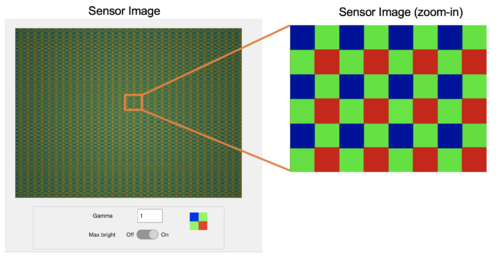
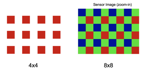
In our experiment, we took images of empty background within the Cornell box. We set the lighting condition to be uniformly distributed so that the original image can be approximated as . In order to minimize the random error, images are captured using different exposure duration, ISO speed, and color channels. In particular, we study the red color channel of captured images. This choice is arbitrary and one may find similar results by using different channels. Note that by selecting a single color channel, we essentially downsample the image to half of its original size.

After the downsampling, we perform standard averaging and normalization for the single-channel image. We then fit a two-dimension surface to the data using Matlab plugin Curve Fitting. We choose a 2D polynomial as shown below:

We then upsample the fitted function back to the original dimension using standard interpolation and renormalize the result to obtain the lens shading matrix . In the code snippet below we show part of our source code that performs the above manipulations.
%% data preprocessing
% Take the mean of raw data to supress noise
mean_data = mean(raw_data, 3);
% Take the red channel (bottom right) by downsampling by two
red_data = mean_data(2:2:end, 2:2:end);
% Normalize data to [0,1]
norm_data = red_data - min(red_data(:));
norm_data = norm_data ./ max(norm_data(:));

%% fit data to 2D polynomial
% Create array indexing
height = size(norm_data, 1);
width = size(norm_data, 2);
[X, Y] = meshgrid(1:width, 1:height);
x = reshape(X, [], 1);
y = reshape(Y, [], 1);
z = reshape(norm_data, [], 1);

% 2D poly fit
sf = fit([x, y], z, 'poly23');
% show fitted function
% % plot(sf, [x, y], z);

% apply fitted function
predicted = sf(X, Y);

%% Upsample to original
% 2D interpolation
[Xq, Yq] = meshgrid(0.5:0.5:width, 0.5:0.5:height);
Vq = interp2(X, Y, predicted, Xq, Yq);

% Normalize the lens shading mask to [0,1]
% mask is of the same size as the original image
% apply elementwise multiplication to apply lens shading
mask = Vq - min(Vq(:));
mask = mask ./ max(mask(:));
Results
Lens Shading
TODO @chien-yi
Lighting Estimation
Real Scene
TODO @wenke add colorbar to grayscale colormap
3D Scene
TODO @wenke add model figures
Conclusions
Reference
[1] A system for generating complex physically accurate sensor images for automotive applications. Z. Liu, M. Shen, J. Zhang, S. Liu, H. Blasinski, T. Lian, and B. Wandell,Electron. Imag., vol. 2019, no. 15, pp. 53-1–53-6, Jan. 2019.
[2] A simulation tool for evaluating digital camera image quality (2004). J. E. Farrell, F. Xiao, P. Catrysse, B. Wandell . Proc. SPIE vol. 5294, p. 124-131, Image Quality and System Performance, Miyake and Rasmussen (Eds). January 2004
TODO @chien-yi


![{\displaystyle M_{ij}\in [0,1]}](https://wikimedia.org/api/rest_v1/media/math/render/svg/c171c38a164353bfdf183dee5e92150f0a66a96d)


