WenkeZhangChien-YiChang

Introduction

The project is to use the graphics model of the Cornell box in ISET3D to simulate the illumination in the box. The project is to adjust the model parameters of the lighting so that the rendered image of the Cornell box matches the relative illumination map measured with the Google Pixel 4a camera. The project was done by Wenke Zhang and Chien-Yi Chang.

Background

In the mid-1980s, researchers at Cornell University compared photographs of a real physical box with computer graphics renderings of the simulated box. It has since been widely used by the computer vision and graphics community for calibrations and other research purposes. The goal of this project is to compare digital camera images of a real physical box with predicted camera images of the simulated box. In particular, we want to adjust the search for parameters of the light model in ISET3D so that the simulated illumination map matches the real image captured by the Google camera. Two steps are required to make the match. The first is to derive a relative illuminant map from the empirical data. We captured images with different exposure times and these can be combined into a single high dynamic range representation. The linear values from the camera, corrected for lens shading, are the target relative illumination map. We will have these images from a few different camera positions. We will use the 3D model of the Cornell box, the spectral radiance of the light, and the reflectance of the white surfaces, to simulate the relative illuminant map in ISET3D. That code produces the spectral irradiance, and we can summarize the spectral irradiance with a single overall value by, say, simulating capture with a monochrome sensor. After that, we can study the effect of lighting parameter models and experiment with different conditions (e.g. type, position, properties) to make the relative illuminant map matches the real as close as possible.

Methods

Overview

Before moving into details, we first discuss the necessary data to create the model using ISET3D. The inputs are i) a 3D model in PBRT of the Cornell box. ii)A mat-file SPD data for light source spectral radiance. iii) The reflectance of the white surface at the interior of the box. Note that these empirical data are provided to estimate the box illumination in Files/Data/Lighting estimation and Files/Data/Lighting estimation (PRNU_DSNU.zip file for lens shading estimation). In addition to these, high dynamic range sensor images (DNG) are obtained using exposure bracketing of the Cornell box with the lighting and white interior. The images will be obtained from different camera positions. We are also provided with camera lens shading data that can be used to calculate the lens shading effect which will be discussed in the following sections. The DNG sensor images are stored in 5 .zip files from 5 different views. They are 'view1.zip' - 'view5.zip'. Each zip file contains a fileinfo.xlsx (Excel) file which summarizes the ISO speed and exposure duration. lightImg.zip file contains several DNG sensor images of the light from the view right below the light window. This file may be helpful for light shape determination. Light spectrum and surface reflectance data are stored in the spectralInfo.zip file.

Figure 1: Cornell box lighting estimation simulation pipeline

Camera Modeling

Lens Shading

Lens shading, also known as lens vignetting, refers to the phenomenon where the light falls off towards the edges of an image when captured by digital camera systems. Lens shading occurs because in the imaging system with an optical lens, the off-axis pixels often receive a smaller bundle of incident rays compared to on-axis pixels, resulting in relatively lower illumination towards the edges. This effect is ubiquitous and not surprisingly can be observed in the data we collected for the Cornell box lighting estimation.

Figure 2. An illustration of the lens shading effect.

In this project, our goal is to accurately estimate the lighting condition for the Cornell box. In order to do this, we first need to deconfound the lens shading effect from the empirical data. One way to achieve this is to preprocess the captured images to remove the lens shading effect and then compared the preprocessed images with the simulated ones. Equivalently, we can apply the artificial lens shading effect to simulated images and then compare it with real images. Here we opted for the latter method.

We first assume that the lens shading effect can be represented as element-wise matrix multiplications

$X_{LS}=X\circ M$, 

where $M$ is the lens shading matrix, $X$ is the original image, and $X_{LS}$ is the image corrected by lens shading effect. We also assume that the lens shading matrix $M$ is of the same dimension as the orignal image $X$, and $M_{ij}\in [0,1]$. The problem is equivalent to finding the lens shading matrix $M$. Once we have found the lens shading matrix, we can apply the lens shading effect to any image by simply multiplying it elementwisly against $M$.

In order to estimate the values of the lens shading matrix $M$, let us consider the case where $X=cJ$, where $J$ is the matrix of ones where every element is equal to one and $c$ is a constant. We have

$X_{LS}=cJ\circ M=cM$, 

and equivalently

$M={\frac {X_{LS}}{c}}$.

Here the left-hand side is the lens shading matrix and the right-hand side is the normalized image with the lens shading effect.

Figure 3. An illustration of camera sensor and pixel arrangement.

In our experiment, we took images of empty background within the Cornell box. We set the lighting condition to be uniformly distributed so that the original image can be approximated as $cJ$. In order to minimize the random error, images are captured using different exposure duration, ISO speed, and color channels. In particular, we study the red color channel of captured images. This choice is arbitrary and one may find similar results by using different channels. Note that by selecting a single color channel, we essentially downsample the image to half of its original size.

Figure 4. By selecting the red channel, we essentially downsample the original image by a factor of two.

After the downsampling, we perform standard averaging and normalization for the single-channel image. We then fit a two-dimension surface to the data using Matlab plugin Curve Fitting [3]. We choose a 2D polynomial as shown below:

We then upsample the fitted function back to the original dimension using standard interpolation and renormalize the result to obtain the lens shading matrix $M$. In the code snippet below we show part of our source code that performs the above manipulations.

%% data preprocessing
% Take the mean of raw data to supress noise
mean_data = mean(raw_data, 3); 
% Take the red channel (bottom right) by downsampling by two
red_data = mean_data(2:2:end, 2:2:end);
% Normalize data to [0,1]
norm_data = red_data - min(red_data(:));
norm_data = norm_data ./ max(norm_data(:));

%% fit data to 2D polynomial
% Create array indexing
height = size(norm_data, 1);
width = size(norm_data, 2);
[X, Y] = meshgrid(1:width, 1:height);
x = reshape(X, [], 1);
y = reshape(Y, [], 1);
z = reshape(norm_data, [], 1);

% 2D poly fit
sf = fit([x, y], z, 'poly23');
% show fitted function
% % plot(sf, [x, y], z);

% apply fitted function
predicted = sf(X, Y);

%% Upsample to original
% 2D interpolation
[Xq, Yq] = meshgrid(0.5:0.5:width, 0.5:0.5:height);
Vq = interp2(X, Y, predicted, Xq, Yq);

% Normalize the lens shading mask to [0,1]
% mask is of the same size as the original image
% apply elementwise multiplication to apply lens shading
mask = Vq - min(Vq(:));
mask = mask ./ max(mask(:));

Light Modeling

Physical Based 3D Scene Rendering

Experiment is set up as a Cornell box with lighting and white interior. Figure 2. (a)-(c) shows object parameters in the physical scene. Then we use 3D software to construct a scene with the same geometry. Exported PBRT file to experiment with different properties: light configurations (including type, position, spectrum, max bounces for the light ray) in ISET3D to make the relative illuminant map matches the real case as close as possible.

Figure 2. (d) shows light image for light shape determination. In the lamp there are three LED lights, a diffuser that blurs the illumination of the three lights at the bottom of the lamp, this give us a direction on how to set up the lighting in the 3D model.

• 

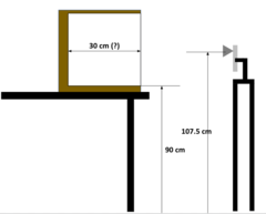  Figure 5. (a) : Cornell box parameters.

• 

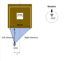  (b) Camera Position.

• 

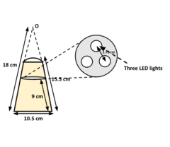  (c) : Lamp Geometry.

• 

  (d) : Light image from the view right below the light window.

Results

Lens Shading

We download the lens shading data from the course website. All lens shading data are stored in the directory named "PRNU_DSNU". Images are taken using the Google Pixel Phone and captured images are stored as .dng files. Images are taken at six different ISOs, ranging from 55 to 798. For each ISO, there are five exposure times, ranging from 0 to 4. We sample five times for each ISO/exposure time combination. We load the .dng files using the ISETCam built-ins and perform data preprocessing as described in the previous section. After the preprocessing, we visualize the normalized image and confirm that the lens shading effect is strong in the raw DNG file.

Figure 6. Lens shading effect as observed in captured DNG files.

We fit the 2D polynomial to the preprocessed data. The result is shown in the image below. We use the fitted function instead of the preprocessed data for the lens shading matrix because we want the matrix to be smooth. As shown in the visualization, even after reducing the noise, the preprocessed data still has a small fraction of rogue data points that cannot be removed. The fitted function, on the other hand, is smooth everywhere so we use it as the final lens shading matrix $M$. We save the matrix in a .mat file for later reusing.

Figure 7. A visualization of the fitted polynomial that is renormalized to produce the final lens shading matrix M

Lighting Estimation

Empirical Data

To derive relative illuminant map from the empirical data, we captured images with different exposure times and these can be combined into a single high dynamic range representation. The linear values from the camera, corrected for lens shading, are the target relative illumination map. We have these images from a few different camera positions.

Figure 8: HDR sensor images (DNG) of the Cornell box obtained with Google Pixel 4a camera using exposure bracketing.

When reading the DNR image, we correct the image with lens shading mask, follow the same procedure to sample the pixel from red channel. Then find the frame with longest exposure time from isospeed file, and on those images, the lighting window would be saturated, so we can identify location of the window. Respectively, for window and box part of the image, we keep the images that are not clipped with saturated value, and normalize each image to unit exposure time, then average across frames.

Then we add the image from window and box into one to derive the target relative illuminant map. Figure shows camera images. Figure the processed images from different camera positions.

Figure 9: Relative illuminant map of HDR image corrected for lens shading.

Simulation

For 3D Scene, input includes: 3D model of the Cornell box exported from cinemas 4d that store the geometry information of the scene, measured the spectral radiance of the light and the reflectance of the white surfaces at the interior of the box. In the 3D model, it has the Cornell box and each camera position with the same parameters as how we taking images. On the top of the window, we test different ways to represent the window and light source, determined by the parameters measured from physical Cornell box and DNG sensor images of the light from the view right below the light window. We then import the PBRT file into ISET3D, edit the recipe, including setting the light spectrum to Box Lamp SPD, apply the material with diffuse reflection color of the walls. Then fine tuning the properties of different light types: spot, area and point light. To simulate the relative illuminant map in ISET3D, we render the scene from PBRT file, it produces the spectral irradiance, then summarize the spectral irradiance with a single overall value by simulating capture with a monochrome sensor, derive the relative illuminant map by subsample the pixels at the same position as the same color pattern in the DNG file.

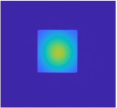
In Figure 10. (a) shows 3D model to simulate the three LED lights as spot light on the top of the window and pointing in the direction of the surfaces. (b) shows the relative illuminant map, it resembles the highlight on the wall and floor.

Figure 10. (a): Spot Lights at the window

Figure 10. (b): Simulated Relative illuminant map of spot lights on the light window.

In Figure 11. (a) shows 3D model to simulate the diffuser at the bottom of the lamp, we use area light with a lower spectrum scale for window, higher spectrum scale for light source. (b) shows the relative illuminant map, as the "diffuse" area light defines an emitter that emits radiance uniformly over all directions in the hemisphere around the surface normal at each point on the surface, with area lights, it is easier to achieve more natural look.

Figure 11. (a): Area Lights on the window

Figure 11. (b): Simulated Relative illuminant map of area lights on the light window.

In Figure 11. (a) shows 3D model to simulate the lamp geometry, we use area light on a sphere shaped light bulb inside the lampshade. (b) shows the relative illuminant map, since we did not measure the material of the lamp, the current model does not has the right reflectance for the shade, as a result, there is less shadow and contrast on the wall, also higher noise in the image.

Figure 12. (a): Area Light with lamp geometry

Figure 12. (b): Relative illuminant map of a sphere shaped area light inside the lampshade.

This is the preliminary result we got from the simulation. It would to be further validated with objects inside the box, and also define metrics to measure the difference between relative illuminant maps.

Conclusions

In this project, we use image systems simulation software (specifically, ISET3D) to create different models for the spatial distribution of light with the simulated Cornell Box. These models are used to predict the amount of light reflected from the walls of the box and from surfaces within the box. We build polynomial model from camera lens shading data to correct HDR images from the lens shading effect, and compare predicted spectral radiance with measurements of spectral radiance obtained.

We experimented with 3D models derived from physical model, the simulation is related but not the same as the camera images. There are simplification we made in each case that could lead to the difference in the relative illuminant map. For the next step, we may want to figure out,

• Is there misuse of ISET softwares?

• Are there important physical properties missing from the current models? we didn't fully understand like objects like diffuser, which could affect light distribution. Would parameter search of lighting properties help?

• Will a black box model works better than replicating physical scene?

• Depends on the goal of this project, is it possible to change the physical light source?

Reference

[1] A system for generating complex physically accurate sensor images for automotive applications. Z. Liu, M. Shen, J. Zhang, S. Liu, H. Blasinski, T. Lian, and B. Wandell,Electron. Imag., vol. 2019, no. 15, pp. 53-1–53-6, Jan. 2019.

[2] A simulation tool for evaluating digital camera image quality (2004). J. E. Farrell, F. Xiao, P. Catrysse, B. Wandell . Proc. SPIE vol. 5294, p. 124-131, Image Quality and System Performance, Miyake and Rasmussen (Eds). January 2004

[3] https://www.mathworks.com/help/curvefit/index.html

Appendix

Psych221 Cornell Box Lighting Estimation project page

Psych221 Cornell Box Lighting Estimation presentation slides

Psych221 Cornell Box Lighting Estimation source code