Wavefront Retrieval from Through-Focus Point Spread Functions with Machine Learning: Difference between revisions
Tag: Manual revert |
|||
| Line 26: | Line 26: | ||
In this project, we use the first 36 Zernike polynomials only. | In this project, we use the first 36 Zernike polynomials only. | ||
== Methods == | == Methods == | ||
Revision as of 22:11, 8 December 2023
Introduction
This project is about estimating wavefront error based on point spread function at different focus locations (at and around focus along optical path). Point spread function can be calculated from wavefront error, but there is no theoretical method to calculate wavefront error from point spread function. This is because the transformation from wavefront error to point spread function is not one-to-one. We overcome this challenge by using machine learning. First, we generated multiple samples of random wavefront error. Second, we calculated the point spread function at a range of focus locations based on each sample of wavefront error. Third, we used regression to relate the wavefront error to point spread function at different focus locations. Lastly, we compared the wavefront error estimated by our regression model to the real wave front error.
Background
Point Spread Function
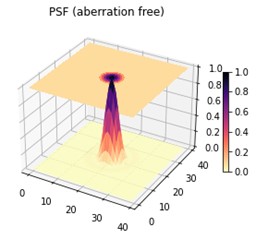
Point spread function can represent optical quality. It is a measure of intensity (or relative intensity) as a function of x and y location (where optical path is along z-axis). Ideally, when a beam pass through a convex lens, the point spread function at focus location should be sharp, where the peak is the location that the beam focuses on.
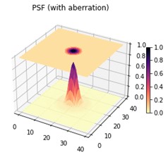
However, with error such as aberration, the point spread function will be flatter.
Wavefront Error
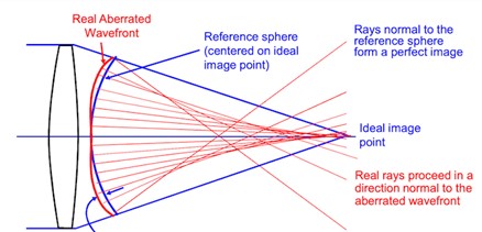
Wavefront error is the difference between the reference wavefront phase and the detected wavefront phase of an optical system.
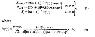
In simulation, we model the wavefront error using Zernike polynomials. Each Zernike polynomial represents the wavefront deviation in shape, and it is orthogonal to other Zernike polynomials. The overall wavefront error can be represented by the sum of a constant multiplying each Zernike polynomial.
Failed to parse (syntax error): {\displaystyle ϕ(u,v)= ∑_1^N c_i Z_i (u,v) } (Zi is a Zernike polynomial)
In this project, we use the first 36 Zernike polynomials only.


