Wavefront Retrieval from Through-Focus Point Spread Functions with Machine Learning

Introduction

This project is about estimating wavefront error based on point spread function at different focus locations (at and around focal length from the lens along optical path). Point spread function can be calculated from wavefront error, but there is no theoretical method to calculate wavefront error from point spread function. This is because the transformation from wavefront error to point spread function is not one-to-one. We overcome this challenge by using machine learning. First, we generated multiple samples of random wavefront error. Second, we calculated the point spread function at a range of focus locations based on each sample of wavefront error. Third, we used regression to relate the wavefront error to point spread function at different focus locations. Lastly, we compared the wavefront error estimated by our regression model to the real wave front error.

Background

Point Spread Function

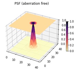
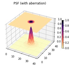
Point spread function can represent optical quality. It is a measure of intensity (or relative intensity) as a function of x and y location (where optical path is along z-axis). Ideally, when a beam pass through a convex lens, the point spread function at focus location is sharp, where the peak is at the location that the beam focuses on.

However, with error such as aberration, the point spread function will be flatter.

Wavefront Error

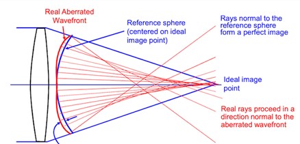
Wavefront error is the difference between the reference wavefront phase and the detected wavefront phase of an optical system.

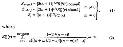
In simulation, we model the wavefront error using Zernike polynomials. Each Zernike polynomial represents the wavefront deviation in shape, and it is orthogonal to other Zernike polynomials. The overall wavefront error can be represented by the sum of a constant multiplying each Zernike polynomial.

$\phi (u,v)=\sum _{i=1}^{N}c_{i}Z_{i}(u,v)$ (Zi is a Zernike polynomial)

In this project, we use the first 36 Zernike polynomials only.

Methods

Set Up

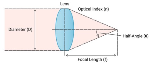
The set up in this project is a beam passing through a lens.

𝑁𝐴=𝑛 sin⁡𝜃

The wavelength of the beam is 550nm. The numerical aperture is 0.65.

We used Python to generate wavefront error samples, calculate the point spread function based on the wavefront error samples and focus locations, derive wavefront error from point spread function, and analyze the results.

Generating Wavefront Error Samples

We used the first 36 Zernike polynomials in this project. We created 500 randomly generated samples of wavefront errors. The wavefront error is represented by an array of 36 Zernike coefficients ($c_{i}$).

$\phi (u,v)=\sum _{i=1}^{36}c_{i}Z_{i}(u,v)$

For each wavefront error, we calculated the point spread function at a range of focus location. Defocus can be expressed by $c_{4}*{\sqrt {3}}(2r^{2}-1)$. We use the unit mWave for focus location and wavefront error. 1 mWave is 1/1000 of the wavelength of light. We experimented on 2 focus location ranges, the first one is -50mWave to +50mWave with 5mWave step, the second one is -500 to +500mWave with 50mWave step. For the range -50mWave to +50mWave, we created several sets of sample based on the total wavefront error magnitude, which are 20, 40, 70 mWave, and 0 – 70 mWave (varying). For the range -500 to +500mWave, we created a set of samples with 0 – 70 mWave (varying) wave front error magnitude. The total wavefront error magnitude is defined by the following equation.

Total wavefront error $(RMS)={\sqrt {\sum _{i=1}^{N}c_{i}^{2}}}$

70mWave is selected, for the reason that the image quality is not sensibly degraded when the total wavefront error is less than or equal to 70mWave RMS.

Calculating Point Spread Function from Wavefront Error

The wavefront error can be expressed in the following form.

$\phi (u,v)=\sum _{i=1}^{N}c_{i}Z_{i}(u,v)$

The point spread function is the modulus square of the Fourier transform of the complex pupil function. It can be calculated from wavefront error with the following method.

$PSF=|F[A(u,v)e^{i\phi (u,v)}]|^{2}$

The implementation is done in Python, and you may refer to the source code for more details.

Generate Training Set

First, an n by n PSF image was calculated at focus F1. Then the image was flattened to n^2 by 1 and normalized by the peak value of PSF w/o aberration. We repeated the steps for all focal positions F1 to FN and got an n^2*N by 1 matrix. Last, we did the same thing for all 500 samples and generated an n^2*N by 500 matrix as the training data.

Regression

The machine learning model we used to estimate wavefront error from point spread function is linear regression. The library “sklearn” from Python was used to execute linear regression. The model was trained with the training data above. We then applied the trained model to predict the wavefront error from the point spread function. The input are the flattened point spread functions through focus. The output are the coefficients of the Zernike polynomials ($c_{i}$). You may refer to the source code for more details.

Analysis

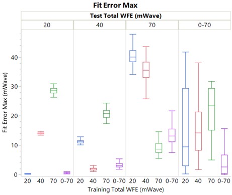
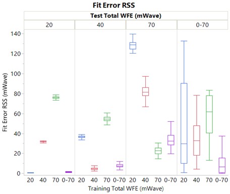
After training our regression model, we computed its accuracy. We used our trained regression model to estimate the wavefront error from the point spread function that we generated earlier for training. We compared the wavefront error estimated by our regression model with the “real” wavefront error that leads to the point spread function. We computed the maximum error among the coefficients of the 36 Zernike polynomials, and the root sum square of the error in those coefficients. Our analysis goal is to verify how close our regression model is in estimating the wavefront error from point spread function.

Results

Range: -50mWave to +50mWave

Fit error max = $max|c_{i,estimated}-c_{i}|$

Where $c_{i}$ is the coefficient of the Zernike polynomial.

$\phi (u,v)=\sum _{i=1}^{N}c_{i}Z_{i}(u,v)$

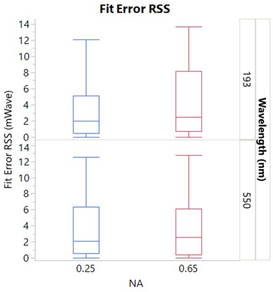
Fit error RSS = ${\sqrt {\sum _{i=1}^{N}(c_{i,estimated}-c_{i})^{2}}}$

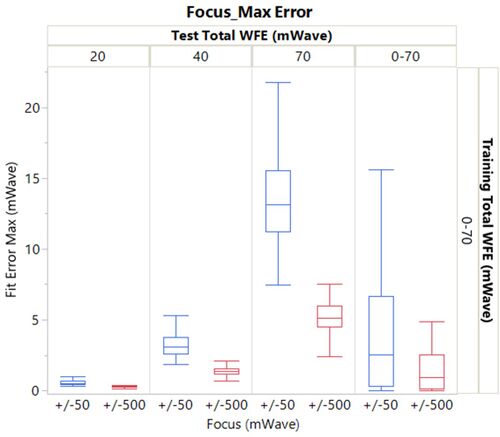
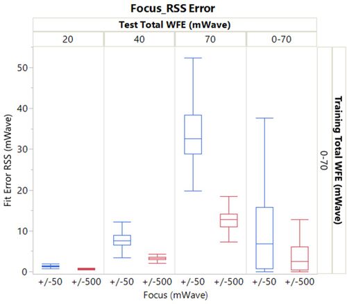
Range of -50 to +50mWave VS -500 to +500mWave

Varying Numerical Aperture and Wavelength

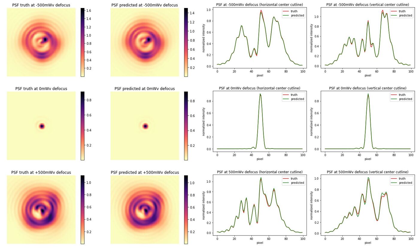
Comparing the Original Image with Image Derived from Estimated Wavefront Error

The following images and graphs compare the original image with the image derived from estimated wavefront error. The training sample has focus range +/-500mWave, and wavefront error range 0-70mWave. The images and graphs are taken at focal length from the lens and +/-500mWave from focal length.

Conclusions

Training our regression model with varying magnitude of wavefront error gives the best overall result (the estimated wavefront error is closer to the real wavefront error). For estimating wavefront error with known magnitude, the regression model trained with that magnitude gives better result. Increasing the focus range gives a better result. Varying the numerical aperture and wavelength has no significant impact on the accuracy of the regression model. If someone is interested to work on the same topic, an alternative is to use deep learning instead of regression.

Reference

https://fakahil.github.io/solo/from-wavefront-aberrations-to-point-spread-function-psf-to-modulation-transfer-function-mtf/index.html

http://kmdouglass.github.io/posts/simulating-microscope-pupil-functions/

http://kmdouglass.github.io/posts/simple-pupil-function-calculations/

Wang JY, Silva DE. Wave-front interpretation with Zernike polynomials. Appl Opt. 1980 May 1;19(9):1510-8. doi: 10.1364/AO.19.001510. PMID: 20221066

Kalinkina, Olga, Tatyana Ivanova, and Julia Kushtyseva. "Wavefront parameters recovering by using point spread function." CEUR Workshop Proceedings. 2020.

Appendix (Source Code)

https://drive.google.com/file/d/1rSv_XhenWuvLQRghCLR4vCCr8IA1JmTT/view?usp=sharing

Appendix (Detailed Training Results)

https://drive.google.com/file/d/1uZdE0v6MUsHJa41Wm68cTt6-PkOtDCir/view?usp=sharing