Rav

Back to Psych 204 Projects 2009

Affect and Choice: Background Information

Imagine deciding which of two equally priced and equally appropriate pictures to buy for a home office. Faced with such a decision, people are thought to consult their feelings and ask, “How do I feel about each option?” (Schwarz & Clore, 2003). A choice between the two affective states is thought to determine which picture is chosen. Now imagine deciding whether to invest in risky high-yield stocks or safer lower-returning bonds. This decision involves considerations that are not purely affective. However, a growing literature suggests that even in such cases affective choice may play a pivotal role in decision making. Indeed, it has been suggested that affect serves as the “common currency” of decision making (Peters, Västfjäll, Gärling & Slovic, 2006). Decision makers decompose complex thoughts into affective states (Mellers, 2000; Pfister et al., 2008) that are then compared with each other, as in the picture example. 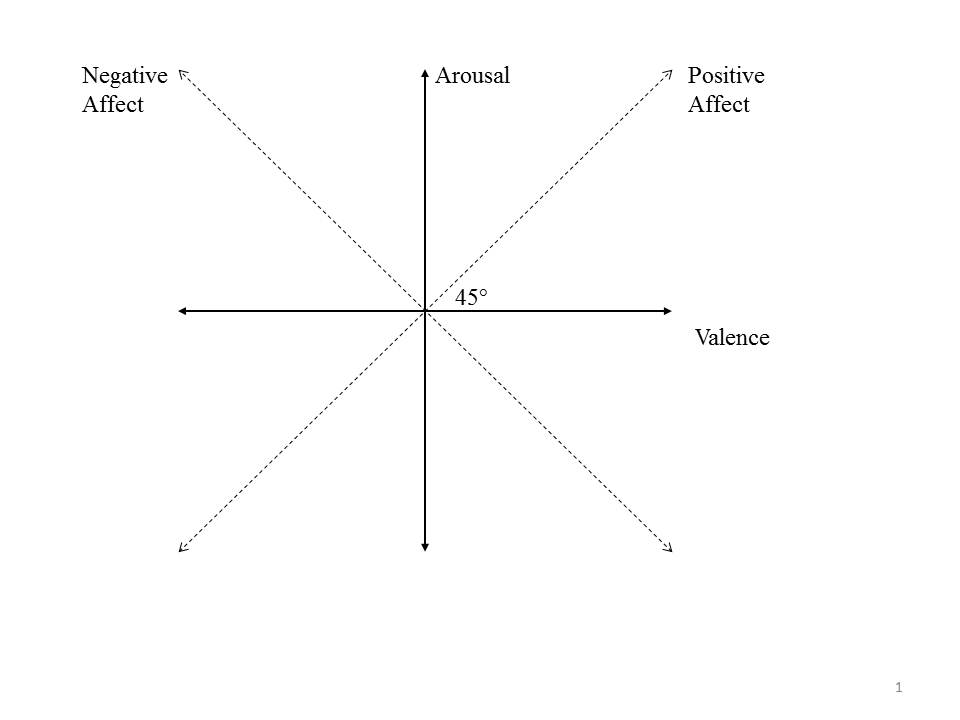Despite the centrality of affective choice to decision making, it is not at all clear how choices between two affective states are made. Our starting point in addressing this issue is a distinction between two fundamental dimensions of affect—valence and arousal. The first, valence, represents the pleasantness/unpleasantness of the affect. The second, arousal, represents the degree of activation associated with the affect. These dimensions capture most of the variance in self-reported mood ratings (Osgood, Suci & Tanenbaum, 1957; Russell 1980; Barrett & Russell, 1999). In addition, cross cultural (Larsen & Diener, 1992), neurobiological (Posner et al., 2009), and developmental data (Russell & Bullock, 1985) demonstrate that – as Wundt (1912) postulated – valence and arousal are core components of affective states. Valence and arousal are often drawn as perpendicular dimensions to create an affective 2-space (Figure 1).

Experiment Structure

60 IAPS pictures (images with affective content) were split into 30 pairs. Within a pair, one picture was designated as Picture 1 and the other as Picture 2. Picture 1 and Picture 2 were counterbalanced for valence and arousal (IAPS population ratings).

In the fMRI, subjects were shown Picture 1 for 500ms followed by Picture 2 for 500ms. They were asked to make a choice between the two pictures. The chosen picture was displayed for 4s—a duration long enough to ensure that the preferred picture was viewed and processed; this attached real affective consequences to each choice.

Outside the fMRI, subjects were asked to rate each image on a 1-7 scale for valence and arousal

Hypothesis

We expected to see 2 sets of results:

1) Distinct areas of the brain would be active for high vs. low valence pictures and for high vs. low arousal pictures. Since a variety of independent sources confirm that valence and arousal are core dimensions of affect, finding neural bases that underlie these dimensions is central to the understanding of affect.

2) We expect activations in these regions to drive choice. In particular a greater positive arousal (PA) would predict choice in cases where both pictures have PA > 0. Similarly in cases where NA > 0, we expect that lower NA would predict choice.

fMRI Methods

Expected Bases of A/V

Based on prior work in the Knutson Lab [1] we expected particular sub-cortical areas to show differential activation:

For Positive Arousal (PA) we expected to see some activation in the Ventral Striatum (Nucleus Accumbens) in particular.

For Negative Arousal (NA) we expected to see some activation in the Insula.

In addition we expected to see some activation in the mPFC for both high valence and arousal pictures.

Subjects

Subjects were 5 healthy volunteers. Results presented here are for a single subject (myself)

MR acquisition

Data were obtained on the CNI scanner at Stanford University. Functional and Anatomicals were reconstructed using CNI algorithms.

AFNI was used to process and analyze the data.

Trial Structure & Shaving of Leading TRs

In this experiment we used the following presentation schedule:

Pic 1: 500MS followed by fixation for 500MS

Pic 2: 500MS followed by fixation for 500MS

Consider Your Choice: 2s

Make Your Selection: 2s

Variable ITI: 2/4/6s

Due to this Trial Structure we chose at TR = 1s.

Further we chose to have 8 leading and 8 trialing TRs to adjust for fMRI start up effects. We eliminated these TRs prior to pre-processing.

Pre-processing

All data were motion corrected, smoothed, drift corrected, normalized and warped.

Motion Corrected

The AFNI command 3dvolreg was used for motion correction.

Smoothing

A blurring kernel of 4mm was used.

Drift Correction

A Fourier highpass filter of 0.011 was used to drift-correct

Additionally:

Data was normalized to percent signal change Anatomical and functional scans were wrapped to talairach space

Post-processing

We used regressors and self ratings to do the analysis.

First we created contrasts (1 0 or 1 0 -1 or parametric) that described the effects.

1,0 -> picture on, picture off

1,0,-1 -> high valence picture, no picture, low valence picture (similarly for arousal)

3,2,1,0,-1,-2,-3 --> exact ratings of valence/arousal deviating from mean 0

Next we convolved the contrasts with the hemodynamic response function

Finally we took the normalized functional data and ran a regression with the contrasts (as long as all contrasts are orthogonal, or aka non-covariance between contrasts). We examined the contrasts in AFNI

Results

Valence

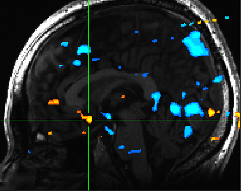
The ventral striatum was reliably activated for positively valenced pictures compared to negatively valenced pictures (Figure 2)

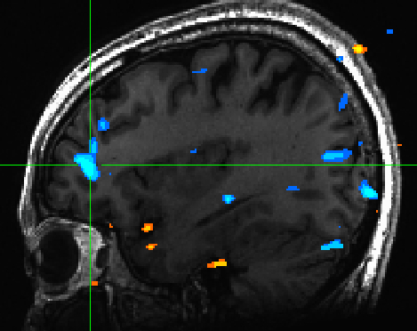
We also saw de-activation in the mPFC for highly valenced pictures -- indicating that low valenced pictures are cognitively processed to a greater extent than high valenced pictures (Figure 3)

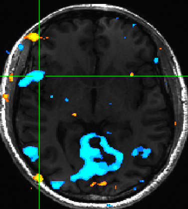
Expectedly we also observed insula activation for negatively valenced pictures (Figure 4)

Retinotopic models in individual subjects transformed into MNI space

Some text. Some analysis. Some figures.

Retinotopic models in group-averaged data on the MNI template brain

Some text. Some analysis. Some figures. Maybe some equations.

Equations

If you want to use equations, you can use the same formats that are use on wikipedia.
See wikimedia help on formulas for help.
This example of equation use is copied and pasted from wikipedia's article on the DFT.

The sequence of N complex numbers x₀, ..., x_N−1 is transformed into the sequence of N complex numbers X₀, ..., X_N−1 by the DFT according to the formula:

$X_{k}=\sum _{n=0}^{N-1}x_{n}e^{-{\frac {2\pi i}{N}}kn}\quad \quad k=0,\dots ,N-1$

where i is the imaginary unit and $e^{\frac {2\pi i}{N}}$ is a primitive N'th root of unity. (This expression can also be written in terms of a DFT matrix; when scaled appropriately it becomes a unitary matrix and the X_k can thus be viewed as coefficients of x in an orthonormal basis.)

The transform is sometimes denoted by the symbol ${\mathcal {F}}$, as in $\mathbf {X} ={\mathcal {F}}\left\{\mathbf {x} \right\}$ or ${\mathcal {F}}\left(\mathbf {x} \right)$ or ${\mathcal {F}}\mathbf {x}$.

The inverse discrete Fourier transform (IDFT) is given by

$x_{n}={\frac {1}{N}}\sum _{k=0}^{N-1}X_{k}e^{{\frac {2\pi i}{N}}kn}\quad \quad n=0,\dots ,N-1.$

Retinotopic models in group-averaged data projected back into native space

Some text. Some analysis. Some figures.

Conclusions

Here is where you say what your results mean.

References - Resources and related work

References

Software

Appendix I - Code and Data

Code

File:CodeFile.zip

Data

zip file with my data

Appendix II - Work partition (if a group project)

Brian and Bob gave the lectures. Jon mucked around on the wiki.