Analysis and Compression of L3 Filters

Project title: Analysis and Compression of L3 Filters

Group members: François Germain, Iretiayo Akinola

Introduction

The L3 algorithm is a learned image processing pipeline for cameras. This new architecture presented by Tian et al. [1] aims at automating the construction of the camera image pipeline that converts a sensor raw image into a displayed XYZ picture. This learned image pipeline is composed of a set of local patch filters that determine the color of an image pixel as a weighted function of the associated sensor pixel and its neighbors.

In its current configuration, the issue is that separate filters are to be learned to deal appropriately with different conditions. As a consequence, the storage requires to store the L3 filters becomes a problem if we want to implement a flexible image pipeline adapted to a large set of scenarios. This project aims at analyzing the structure of the L3 filters and discover methods allowing to efficiently store and interpolate an entire bank of filters from a reduced set of values. Such findings are an important step towards improving the usability of the method in practical settings, where we have a limited amount of computation power and storage space, as it would be the case in current cameras.

L3 filters

The L3 (Local, Linear and Learned) method builds the observations that there are some local linear relationship between sensor responses (voltage levels) and scene statitics (XYZ value) by trying to empirically learn these local transform through a machine learning algorithm. As a consequence, we can learn a set of transforms that will incorporate all the components of the image pipeline (demosaicing, denoising, etc...) in a set of filters. A new scene is then be decomposed into patches around each pixel, each of these pixels is matched with the filter corresponding to the patch characteristics, and the resulting XYZ pixel on the rendered image is obtained by applying those filters to the patch.

Training the L3 filter bank

To train the L3 filters, the learning algorithm is given a set of training patches spanning the desired characteristics (see filter structure below). For each training patch, we have its ideal (noise-free) pixel value, and we can then tune the filters in order to minimize the difference between the results of the processing of the patch by the filters, and the actual (ideal) pixel value.

L3 filter training process. Reproduced from [1].

L3 filter bank structure

The L3 algorithm aims at learning the filters spanning a variety of conditions regarding the input sensor image, as we expect different conditions to lead to . The different parameters are as follows:

• Illuminant (D65, Tungsten, etc...): We know [2] that humans are quite good at perceiving color in a scene independently of the color introduced by the light illuminating that scene. As a consequence, the color perception of such scene does not match the actual color in the scene (due to the coloration added by the illuminant). To deal with this phenomenon, the camera image pipeline needs to embed illuminant correction in the filter bank to transform the sensor values of an image under a given illuminant into a displayed image with colors under a reference (white) light. This implies that a set of filters is unique to a given illuminant as the illuminant correction is embedded inside the filters themselves. In the L3 setup, the reference light is chosen to be D65.
• Patch type: A given image pixel is built by integrating a square patch of sensor pixels around that same pixel (the center pixel) in the sensor array. Depending on the position of this center pixel on the sensor, we will get different pixel configurations for the patch {figure!}. For this reason, we get a set of filters for each patch type on the sensor.
• Luminance level: Luminance is strongly correlated to the amount of photon noise we expect to experience in the sensor levels. For high noise environment, we expect to need to average several pixels on the sensor in order to reduce that noise (at the price of image sharpness), while for low noise, the center pixels of a patch on the sensor should be enough to compute the color values of the image (without losing sharpness). In order to capture this behavior, a different set of filters is learned for each luminance scenario. For practical purposes, the luminance dimension has to be quantized in "bins", and a given sensor patch is meant to be matched to the luminance bin it belongs to when picking the patch.
• Saturation configurations: When a pixel gets saturated in the sensor, its contribution to the image often has to be discarded and the image pixel value has to be infered from the remaining non-saturated pixels, leading to a different set of filters for each saturation configuration {figure!}.
• Spatial Contrast ("flat"/"texture"): A different set of filters is stored depending on the spatial contrast of the patch. "Flat" patches are relatively uniform image areas that contain only low spatial frequencies. Texture patches contain higher frequencies, typically near an edge.
• Color channels (X,Y,Z): For each patch, we need to store one filter for each output color channel.

L3 filter class structure for a given illuminant with an RGBW configuration. Each class will contain a filter for each color channel (X,Y,Z). Reproduced from [1].

Dimensionality

In the L3 filters provided to us by Qiyuan T., a typical filter bank for a given illuminant would have:

• 4 patch types (as current CFA patterns are 2x2)
• 20 luminance levels (with finer sampling at low luminance levels)
• 6-8 saturation configurations
• 2 contrast types ("flat"/"texture")
• 3 color channels (XYZ)

From these statistics, we expect a filter bank to contain up to 3840 independent patches. In practice, we get about 50% of such filters because of the fact that some luminance levels will not display some of the saturation conditions (e.g. at low luminance levels, we won't observe more than 1 saturated sensor pixel type). For our setup, a patch has a 5x5 pattern, resulting in around 45,000 values to store for a given illuminant. This dimensionality would then increase further if we add the fact that it would be desirable to be able to store at least 10 different illuminants.

Project objectives

Our project aims at analyzing the L3 filter bank in order to discover potential methods allowing to reduce the dimensionality of the filter bank, and allow it to be practically embedded on a camera. This dimensionality reduction should come at the cost of limited introduced distortion (color, noise,...) in order to validate a given approach. As this is a preliminary exploration, the presented methods will be mostly linear, but this is desirable feature as we would want to limit the computional load required to recover a compressed dimension.

Methods

In our project, we have focused on reducing dimensionality across two quantities where we expected strong correlations between different L3 filters. These two dimensions are:

• Compression of the Illuminant correction process
• Compression across luminance levels

Provided data and code

All the rendering process used in this project relies on the functions provided as parts of iset-camera.

In addition, Qiyuan T. provided us with the following data:

• The L3 filters trained with the following parameters:
  • 9 illuminants (D50, D55, D65, D75, Fluorescent, Tungsten, Illuminants A, B and C)
  • 20 luminance levels
  • 2 types of CFA geometry (Bayer and RGBW)
• 14 scenes stored in multispectral form

These L3 filters were provided as part of camera objects used in ISET to simulate the capture, processing and rendering of an image by a virtual camera. In the current structure, a different camera object is used for each illuminant. In addition to those cameras, we were also provided with a single camera object for D65 light and RGBW geometry with 180 luminance levels.

In addition, Qiyuan T. provided us with the scripts necessary to:

• Extract the raw sensor data for a given picture with a given camera object (meaning the used illuminant corresponds to the one in that object)
• Render the displayed image after processing of the sensor data by the L3 filter bank
• Compute an ideal image (noise-free and without illuminant correction)

Illuminant correction

While various illuminants exist, the D65 illuminant is widely accepted as the standard illuminant for visual appeal. Hence, images in other illuminants are sometimes converted to their D65 version. Using L3, the raw image sensors from the "alien" illuminant is passed through a pipeline of filters which transforms the image to the D65 version. This meant that a complete set of trained filters was stored for each illuminant (CIE standard illuminants include D65, D50, Tungsten,. The latter shows the spectrum of tungsten (incandescent) light in red, and fluorescent).

As mentioned in the introduction, the L3 filter architecture embeds the illuminant correction process in the filter bank associated with that illuminant (blue arrow). The resulting process is shown in the next figure where the sensor image for a given image has to be processed by the corresponding filter bank in order to compute the image under the reference light (here D65). In this project, we have investigated 3 approaches aiming at replacing the entire illuminant-corrected filter bank of an alternative illuminant (blue arrow) by a simple linear transform that would then be associated with the L3 filter bank of the reference light in order to achieve the desired illuminant correction on the captured scene. We would then only need to store the filter bank associated with the reference (D65) light and a linear transform associated with each illuminant we want to integrate in our framework.

L3 processing on sensor image with (green arrow) and without (blue arrow) illuminant correction. The objective of this project is to avoid having to store the filters associated with the blue arrow (with illuminant correction)

As mentioned by Steven L. during our project, the convention we use in order to render images without illuminant correction under any illuminant is done by using the L3 filters associated with the reference light. Indeed, no significant difference was observed between the filter banks of the reference light, and the filter banks built without illuminant correction for all of the lights. This is why the filter bank used to go from left to right will always be the one of the reference light (green arrow).

Method 1 - XYZ image processing

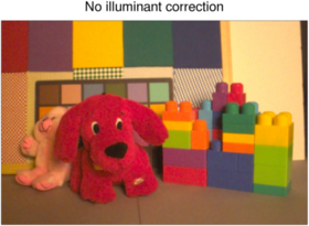
In our first approach, we look at replacing the illuminant correction by the following process: 1) the sensor image is processed without illuminant correction using the reference light filter bank (green arrow), and 2) the rendered XYZ image is transformed to correct for the illuminant (red arrow).

Method 1: The sensor image is first L3-rendered without illuminant correction (green arrow), followed by a linear transformation on the XYZ image (red arrow)

To perform the second step, we look for a linear correlation between the computed images in the XYZ domain under the reference light and under the alternative illuminant. Since we expect the three color channels to be correlated, we look to find a full 3x3 linear tranform ($C$) between the pixel value of the reference ($P_{Ref}$) and the alternative illuminant ($P_{Alt}$) according to the formula $P_{Ref}$ = $C$ x $P_{Alt}$ or alternatively:

${\begin{bmatrix}P_{X}\\P_{Y}\\P_{Z}\end{bmatrix}}_{Ref}={\begin{bmatrix}C_{XX}&C_{XY}&C_{XZ}\\C_{YX}&C_{YY}&C_{YZ}\\C_{ZX}&C_{ZY}&C_{ZZ}\end{bmatrix}}_{Alt\rightarrow Ref}{\begin{bmatrix}P_{X}\\P_{Y}\\P_{Z}\end{bmatrix}}_{Alt}$

That transform should be independent from any feature of the image (luminance,...) besides the capture light. With the scripts provided by Qiyuan T., we actually have several options regarding which image data we can use as points for the fit. In our study, we explored the following combinations:

	Reference light image	Alternative light image
1)	Ideal image under reference light	Ideal image under alternative light
2)	L3-rendered image under reference light	L3-rendered image under alternative light without illuminant correction
3)	L3-rendered image under alternative light (with embedded illuminant correction)	L3-rendered image under alternative light without illuminant correction

In the 3 cases, the transformation matrix is estimated with least-squares fitting on the data points.

Method 2 - Filterbank adaptation

In our second approach, we look at replacing the illuminant correction by the following process: 1) the filter bank of the reference light ("without illuminant correction" - green arrow) is transformed into a filter bank embedding the illuminant correction (black arrow), and 2) the sensor image under the alternative light is rendered using this filter bank (red arrow).

Method 2: The reference light filter bank is adapted to include the illuminant correction for the corresponding light (black arrow), followed by the rendering of the sensor image with the adapted filter bank (red arrow)

We now need to look at linear correlations between the filter bank of the reference light and the one of the alternative light. To do so, we go though the different dimensions (luminance, saturation, patch type, color channel and contrast) and collect all the filter values corresponding to a given sensor pixel color. For example, in a Bayer mosaic, we will group together all the filter values associated respectively with R, G and B pixels across the 4 patch types, the 3 color channels (X,Y,Z) and the 2 contrasts (flat/texture). The idea is to discover if there is a linear relationship between a pixel of a given color in the reference light filter bank and its counterpart, meaning that we can find a set of coefficients $C$ (one per sensor pixel color). In the case of a Bayer mosaic, we would then have 3 coefficients $C_{R}$, $C_{G}$ and $C_{B}$ such that all the pixels of a given color filter (whichever filter they belong to in the reference light filter bank) will be rescaled by the corresponding transform coefficient in order to approximate the alternative light filter bank (blue arrow). It is important to notice that since the filter patches are composed of sensor pixels with their unique color filter, we shouldn't observe any correlation between pixels of different colors.

The coefficients are estimated using weighted least-squares. Indeed, we expect the L3 filter values to be more noisy if their intensity is small, as signal-to-noise ratio decreases at low light intensity. Hence, we want to give a larger weight to pixels with large values during the fit since we expect those to be more reliable (less noisy).

Method 3 - Raw data processing

In our third approach, we look at replacing the illuminant correction by the following process: 1) the pixels of the sensor image under the alternative light are rescaled to correct for the illuminant , and 2) the re-scaled sensor image is rendered using the filter bank of the reference light wihout illuminant correction (green arrow).

Method 3: The sensor image is first reweighted to simulate the reference light (red arrow), followed by the L3-rendering without illuminant correction (green arrow).

For that last part, we look at the linear correlation between the sensor pixels of a given color filter under both lights. For example, we would like to discover if we can find a linear relationship between the voltage levels of a given red sensor pixel for a given picture under both lights. We can then store a set of coefficients $C$ (one per sensor pixel color). In the case of a Bayer mosaic, we would then have 3 coefficients $C_{R}$, $C_{G}$ and $C_{B}$ such that all the pixels of a given color filter (wherever they are located on the sensor) will be rescaled by the corresponding transform coefficient in order to approximate the sensor response under the reference light. Again, since we are working on sensor pixels with their unique color filter, we wouldn't expect to observe any correlation between pixels of different colors.

For the same reason as in the second method, we will use weighted least-squares to fit the different coefficients.

Compression across Luminance levels

In this part of the project, we aim at exploiting linear relationships between different luminance levels in order to store some of this levels as linear functions of others. More exactly, our approach is to search for segments of contiguous filters with a reasonable linear relationship between them and replace with weighted versions of the two extremal filters of that segment. The implication of this is that all intervening filters can be replaced by two weights in terms of the two filters at the boundaries. To do so, we sweep along the luminance dimension of the filters in order to find and compress filters exhibiting such relationships. The test for linear dependence was done using the SVD analysis; and a new filter is judged linear dependent on the existing ones if it does not increase the number of principal components of the set. A threshold is set for the ratio of the Frobenius norm of the new matrix to the old full matrix. The threshold aims at limiting the error between the recovered filters to the original set below perceptible effects of the picture output. At the end of the algorithm, we record the amount of compression as the number of filters that were replaced by (2) linear weights.

Illustration of the algorithm. The centre filter is replaced by two weights which can be used to recover it when needed.

The method follows:

• Sweep along the luminance dimension of the L3 filter bank
• Find a contiguous set of three filters coefficients and using SVD analysis check if there are two principal components. The ratio of the square of the third singular value to the norm of the vector of all singular values is compared to a set threshold. If it is less than this threshold, there's a reasonable linear dependence among the filters. The choice of threshold was arbitrary and the performance using different thresholds were compared.
• The range of the compared filters expands until this test for linearity fails. For a range of linearly dependent filter, the boundary values are stored while two weights are stored for the intervening filters.
• Then the cycle is repeated for the next set of filters starting the end point of the previous boundary.

This form of storage has a little extra computation cost of recovering the filter but, but we expect the simplicity of the operation to be compensated by significant storage savings. This method was carried out on dataset that had been quantized into 20 luminance levels with findings discussed below in Results sections. A question naturally arise regarding this compression scheme, when we need to judge how good are the original choices for the location of the luminance levels. Put differently, how could we optimally choose the quantization for the luminance levels so as to minimize at once the distortion of the L3 pipeline and the number of stored filters. The next section describes an approach to answer this question.

Clustering to determine Luminance (Quantized) Levels

In the L3 scheme, separate classes are created along the luminance level axis, effectively quantizing it to a limited number of bins. These classes are expected to deal with the variation of image pipeline treatment of the sensor response level as the signal-to-noise ratio (SNR) varies greatly with luminance. In Tian et al. [1], the classes along the luminance axis (quantization) is based on a more densely sampled dimension for lower response levels are more densely sampled, under the assumption that the SNR changes rapidly in that range[1]. While this is a very reasonable assumption, we decided to investigate a posteriori the correctness of that assumption. Starting with filters trained filters for 180 different luminance levels (dense luminance sampling), we run a greedy search in order to merge neighboring levels into a luminance band while minimizing the added distortion at each merging step.

Algorithms:

• Each of the luminance levels are placed in a different individual cluster.
• The square error of matching one cluster to the next is calculated for all clusters. Each cluster is assumed to take on the filter values of its mid-point (the middle of the implied quantization band). The error of merging one cluster to another is set to be the large squared distance between the filters in the band and the mid-point filter.
• We perform the merging for which the least possible error was recorded.
• This previous two steps are repeated until the predetermined number of quantized levels is reached.

We end up with a set of luminance level bands that can be used as positioning for the luminance levels for the L3 learning algorithm. In practice, we simulate such learning by creating a L3 filter structure where all the filters associated with a given luminance band are copies of the mid-point filter of that band, so that the rendering algorithm will emulate the situation where the new set of quantized band was being used.

Results

In this section, we present a few results from the application of the ideas exposed in the methods section. The sections are organized in the same order.

Illuminant correction

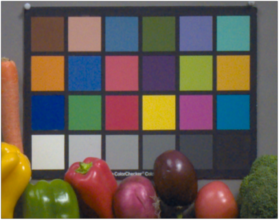
In this section, we present the results of our experiments using the methods presented above. In our setup, we use the D65 illuminant as reference, as it is the one chosen by Qiyuan in his implementation of the L3 algorithm. This is motivated by the fact that D65 is widely accepted as the standard illuminant for visual appeal. Hence, L3 convert images in other illuminants to their D65 version by using illuminant correction. Here, we will use the Tungsten illuminant as alternative illuminant as its spectral distribution differs significantly from the D65 illuminant, resulting in a significant illuminant correction.

Method 1 - XYZ image processing

Here, we try to find a linear transform between the XYZ images rendered under different illuminants without correction.

Transform estimation

To compute the 3x3 tranform matrix, we render the 14 images we have using 1) L3 rendering under D65 light, 2) L3 rendering under Tungsten light (with illuminant correction), and 3) L3 rendering under Tungsten light withouth illuminant correction under 3 mean luminance conditions (10, 30 and 80). To perform 3), we have to replace the filters in the camera object associated with Tungsten light by the ones contained in the camera object associated with D65 light.

As mentioned earlier, we can use different sets of pictures to estimate our transform matrix. For the 3 methods, we obtain the 3 following matrices:

Estimation method (see "Methods"):	1	2	3
	${\begin{bmatrix}0.6273&0.2215&0.2154\\-0.2560&1.271&0.0794\\0.0787&-0.1059&2.6409\end{bmatrix}}$	${\begin{bmatrix}0.5738&0.2909&0.1905\\-0.2842&1.3106&0.0703\\-0.2217&0.275&2.3927\end{bmatrix}}$	${\begin{bmatrix}0.5625&0.4042&-0.0553\\-0.3641&1.5199&-0.228\\-0.1133&0.1448&2.4106\end{bmatrix}}$

As expected, we see that the coefficients obtained from each method are quite similar.

Image example

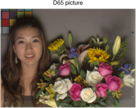
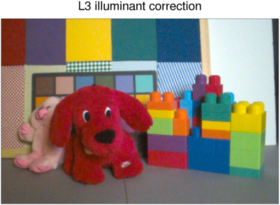
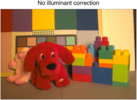
An example of illuminant correction in the XYZ domain is provided in the figure below. As target, we render the scene under D65 light with the L3 filters (Fig. (a)), as well as under Tungsten light with the illuminant-corrected L3 filters (Fig. (b)). The objective here is to see if by applying the transform matrices given above, we can post-process the scene as rendered under Tungsten light without illuminant correction (Fig. (d)) and achieve illuminant correction. The results using the three matrices are given in (respectively) Figs. (c), (e), and (f).

• Illuminant correction in the XYZ domain
• 
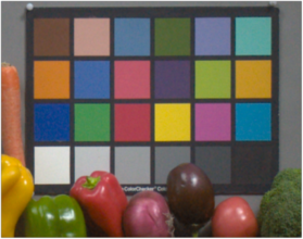  (a) Target image
  L3-rendered image under D65 light
• 
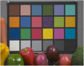  (b) Original L3-rendered image under Tungsten light
  (with illuminant correction)
• 
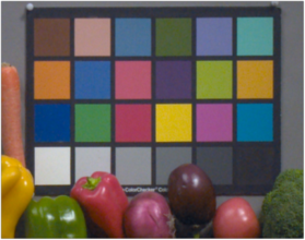  (c) L3-rendered image under Tungsten light without correction and post-processed by matrix no.1
• 
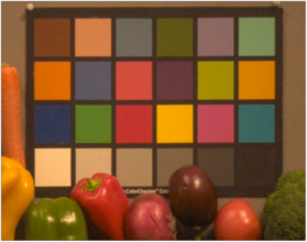  (d) L3-rendered image under Tungsten light
  without illuminant correction
  
• 
  (e) L3-rendered image under Tungsten light without correction and post-processed by matrix no.2
• 
  (f) L3-rendered image under Tungsten light without correction and post-processed by matrix no.3

As we can see, the linear transform in the XYZ domain is quite efficient at achieving illuminant correction. Of the 3 matrices, matrix no.1 seems to be the best, as the two other ones slightly wash out the colors (Figs. (e) and (f) are a bit whiter). Hence, the 9 coefficients of any of those matrices are sufficient information to perform a convincing illuminant correction.

Method 2 - Filterbank adaptation

In this case, we try to find a diagonal linear transform between the RGB pixel values of the L3 filter banks of the reference illuminant and the alternative illuminant.

Transform estimation

For this method, we have looked at two different sensor mosaics (Bayer and RGBW) in order to discover a linear relationship between the values of the pixels of a same color in all the filters of the D65 ligth (reference) and the illuminant-corrected Tungsten light (alternative).

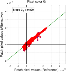
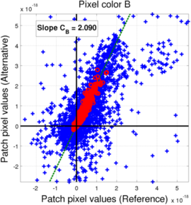
• Filter color pixel value for Bayer mosaic - D65 vs. Tungsten
• 
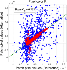  (a) Red pixels (blue: All saturation levels, red: non-saturated level)
• 
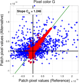  (b) Green pixels (blue: All saturation levels, red: non-saturated level)
• 
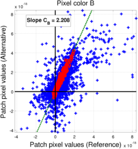  (c) Blue pixels (blue: All saturation levels, red: non-saturated level)

In the case of the Bayer mosaic, if we compared the values of the pixels for all the saturation levels (blue points), we observe a significant scattering of the points, meaning it is quite unlikely that the relationship between the two filter banks could be explained with a simple transform. However, we can see that the non-saturated filters actually do mostly align along a line, meaning we can derive a linear relationship (through weighted least-squares as explained earlier). The behavior for the saturation levels can be explained by the fact that color reconstruction in a Bayer mosaic with a pixel missing a rather difficult, so the L3 processing for such cases becomes non-linear, leading to the observed scattering. As a consequence, we will use the coefficients extracted from the non-saturated filters as our transform coefficient.

• Filter color pixel value for RGBW mosaic - D65 vs. Tungsten
• 
  (a) Red pixels (blue: All saturation levels, red: non-saturated level)
• 
  (b) Green pixels (blue: All saturation levels, red: non-saturated level)
• 
  (c) Blue pixels (blue: All saturation levels, red: non-saturated level)
• 
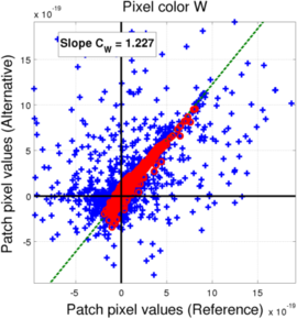  (c) White pixels (blue: All saturation levels, red: non-saturated level)

In the case of the RGBW mosaic, we also see that the linear relationship is valid only for non-saturated cases. However, we see that the linear relationship is not always valid. In particular, we can notice a slight elbow on the red pixel value distribution. This is probably due to the fact that since we have one more pixel color (W) whose response overlaps all the other ones, the distribution of the pixel values is not unique. Depending on the situation, the L3 learning algorithm can then priviledge one or the other. As approximation, we still get an estimation of the transform by looking at the weighted least-squares fit along the non-saturated filters.

The resulting coefficients for the conversion between D65 and Tungsten light L3 filters are presented in the following table:

Conversion coefficients - D65 to Tungsten light
Pixel color	Bayer	RGBW
R	0.776	0.778
G	1.249	0.817
B	2.059	1.162
W	/	1.712

Illuminant correction example

An example of illuminant correction by filterbank adaptation is provided in the figure below. Here we want to compare the correction of the Tungsten light achieved by the original L3 filters with illuminant correction (Fig. (c)) with the one by the L3 filters adapted from the L3 filter bank of the D65 light (Fig. (b)), in order to match a picture rendered under D65 light (Fig. (a)). For reference, we also have the image rendered under Tungsten light without illuminant correction (Fig. (d)). One set of image is given for each mosaic type.

• Illuminant correction by filter adaptation for Bayer mosaic
• 
  (a) Target image
  L3-rendered image under D65 light
• 
  (b) L3-rendered image under Tungsten light with a L3 filterbank adapted from the D65 filterbank
• 
  (c) Original L3-rendered image under Tungsten light
  (with illuminant correction)
• 
  (d) L3-rendered image under Tungsten light
  without illuminant correction
  

• Illuminant correction by filter adaptation for RGBW mosaic
• 
  (a) Target image
  L3-rendered image under D65 light
• 
  (b) L3-rendered image under Tungsten light with a L3 filterbank adapted from the D65 filterbank
• 
  (c) Original L3-rendered image under Tungsten light
  (with illuminant correction)
• 
  (d) L3-rendered image under Tungsten light
  without illuminant correction
  

In both cases, we observe that a significant part of the light coloration from the Tungsten light was removed. However, the adapted filter banks do not entirely remove it, resulting in pictures with a slight yellow coloration. Hence, only a few coefficients (3 for Bayer, 4 for RGBW) are sufficient information to perform a convincing illuminant correction.

Method 3 - Raw data processing

In this case, we try to find a diagonal linear transform between the RGB pixel values of the captured sensor image under the reference illuminant and under the alternative illuminant.

Transform estimation

To estimate the parameters of our transform, we look at the matching between the sensor pixels for a given pixel color for D65 (reference) and Tungsten light. The pixel values are collected on the 14 scenes we have, for a mean luminance level of 30 in order to avoid a too strong photon noise while limiting the number of saturated pixels. In our (weighted) least-squares fitting, we remove from the data points:

• pixels for which the voltage level under either light is 0
• pixels for which the voltage level under either light is saturated ("1" in normalized scale)

This matching is displayed in the following figure:

• Filter color pixel value for Bayer mosaic - D65 vs. Tungsten
• 
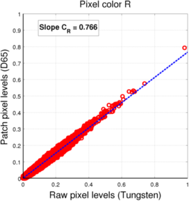  (a) Red pixels
• 
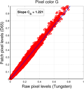  (b) Green pixels
• 
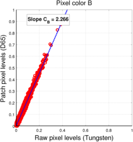  (c) Blue pixels

• Filter color pixel value for RGBW mosaic - D65 vs. Tungsten
• 
  (a) Red pixels
• 
  (b) Green pixels
• 
  (c) Blue pixels
• 
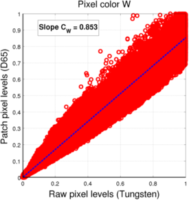  (c) White pixels

For both mosaics, we see that the pixel values under each light (for a given pixel color) are located roughtly along a line, which means we can assume the linear fit to be a valid approximation of the relationship between one sensor value and the other.

The resulting coefficients for the conversion between D65 and Tungsten light L3 filters are presented in the following table:

Conversion coefficients - D65 to Tungsten light
Pixel color	Bayer	RGBW
R	0.766	0.766
G	1.221	1.222
B	2.266	2.267
W	/	0.853

It is interesting to notice that the coefficients in the case of the Bayer mosaic are very close to the coefficients we got for the filter adaptation in the second method. This is probably due to the fact that the R, G, and B channels are relatively decorrelated, leading to similar transforms at the level of the sensor and the level of the filter patches. In the case of the RGBW mosaic, it is no longer the case, which can be easily interpreted as the fact that the four channels contain redundant color information (4 input color channels for only 3 output color channels). This was also the reason why, in the filter adaptation, the linear relationship between the filter coefficients was not always conserved as the optimal mixing of input color channels should not be unique anymore.

Illuminant correction example

An example of illuminant correction by raw sensor image processing is provided in the figure below. Using the estimated coefficients from the previous section, we can reweights the sensor pixels in order to correct for the light at the raw sensor image level. Here we want to compare the correction of the Tungsten light achieved by the original L3 filters with illuminant correction (Fig. (c)) with the one achieved by processing the reweighted sensor image with the D65 L3 filter bank (Fig. (b)), in order to match a picture rendered under D65 light (Fig. (a)). For reference, we also have the image rendered under Tungsten light without illuminant correction (Fig. (d)). One set of image is given for each mosaic type.

• Illuminant correction by sensor image processing for Bayer mosaic
• 
  (a) Target image
  L3-rendered image under D65 light
• 
  (b) L3-rendered image under Tungsten light with the D65 L3 filterbank after reweighting the sensor image
• 
  (c) Original L3-rendered image under Tungsten light
  (with illuminant correction)
• 
  (d) L3-rendered image under Tungsten light
  without illuminant correction
  

• Illuminant correction by sensor image processing for RGBW mosaic
• 
  (a) Target image
  L3-rendered image under D65 light
• 
  (b) L3-rendered image under Tungsten light with the D65 L3 filterbank after reweighting the sensor image
• 
  (c) Original L3-rendered image under Tungsten light
  (with illuminant correction)
• 
  (d) L3-rendered image under Tungsten light
  without illuminant correction
  

For both mosaics, we can observe that our processing corrects convincingly for the illuminant. By comparing images (b) and (c), we see a few differences in the treatment of some of the colors (especially red/magenta) but both are quite good at approximating the target image under D65 (Fig. (a)). Hence as for filter adaptation, only a few coefficients (3 for Bayer, 4 for RGBW) are sufficient information to perform a convincing illuminant correction.

Compression across Luminance levels

Here we present some of the results of the compression across Luminance levels as described in Methods section above.

As suspected, we find some levels of redundancies existed between filters for different luminance levels, as it is visible on the figure on the left representing the evolution of the filter pixel values as luminance varies (The figure on the right gives an illustration of what each line of the plot represents). For the 5x5 patch, there are 25 line plots on that figure though some completely overlap.. The different straight line portions of a plot of filter coefficients reveals correlations that can exploited to store the filters more compactly. Our approach is then to search for contiguous filters with a reasonable linear relationship between them and replace with a line.

• 
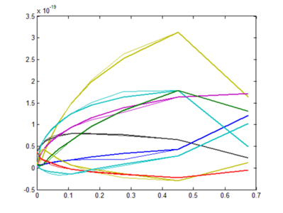  Plot of one of the uncompressed filters along the luminance dimension
• 
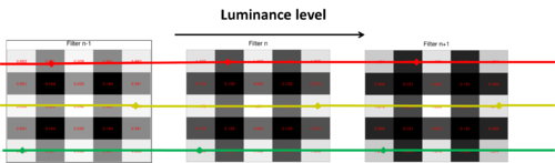  Illustration of what each line in the left plot represents.

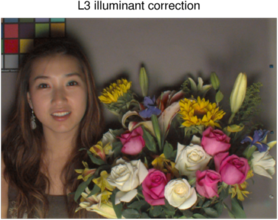
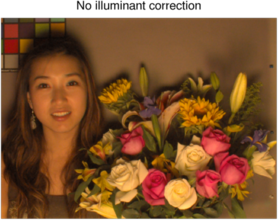
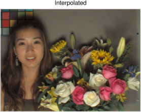
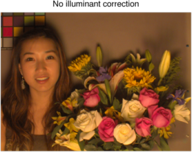
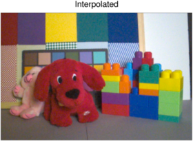
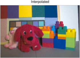
In our experiments, the filter is first compressed and stored using the algorithm described in the methods section. Then the full filter is reconstructed from the compressed version by interpolating the compressed points using the stored weights. The performance of the original filter bank is compared with the interpolated version by overlapping the plots of the filter coefficients for original and compressed filters. The comparative plots reveal that there is a significant match with minimal errors for compression ratio superior to 50%. In the figures below, the thin lines represent the original filter coefficients of the original filter bank while the thick lines show the recovered values from interpolation of the compressed version. Images are rendered for both versions of the filter (compressed and non-compressed) in order to evaluate the introduced distortion.

The figures below show the filter coefficient plot and rendered image for each of the compression levels.

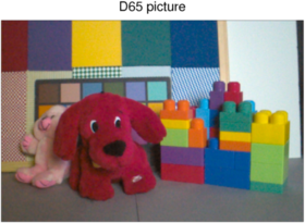
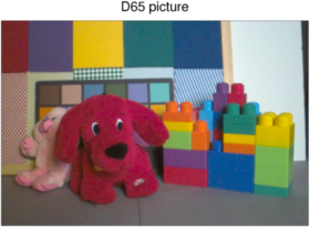
• Comparison of Rendered Images for the Interpolated Filters from different degrees of Compression
• 
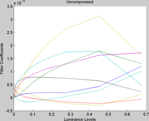  Plot of Original Filter coefficients across luminance levels
• 
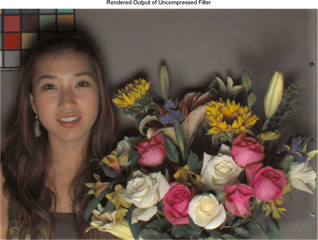  Rendered Image using Uncompressed filter bank
• 
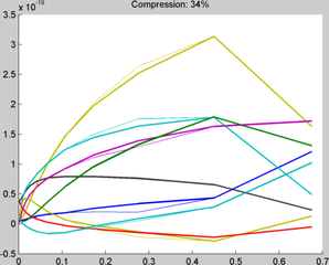  Plot of Interpolated Filter coefficients across luminance levels (34% compression)
• 
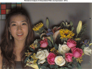  Rendered Image using Interpolated filter bank after 34% compression
• 
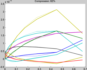  Plot of Interpolated Filter coefficients across luminance levels (62% compression)
• 
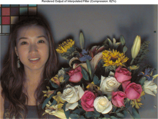  Rendered Image using Interpolated filter bank after 62% compression
• 
  Plot of Interpolated Filter coefficients across luminance levels (75% compression)
• 
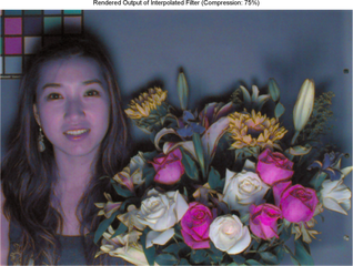  Rendered Image using Interpolated filter bank after 75% compression

As mentioned earlier, the critical factor in this algorithm is determining if a cluster of points are linearly dependent and replacing the the intervening points of cluster with two weights of the boundaries values. A threshold is usually set for the maximum ratio of the square of third singular value to square of norm of the entire vector of singular values to ensure that the cluster has approximately two principal components. As mentioned in the methods section, the compression value is estimated as the ratio of filters which are replaced by relative weights. The effect of varying the threshold value from 0.005, 0.0005, 0.00005 is a compression of 75%, 62%, 34% respectively. At 62% compression, the rendered image looks very similar to the original one with only small distortion. Increasing the compression beyond this point resulted in visible distortion in the rendered image.

Clustering to determine Luminance (Quantized) Levels

Starting with a large dataset trained for 180 different luminance levels, we decided to cluster filter coefficients into groups where each group is treated as one luminance level all taking the filter coefficient values of the midpoint of the cluster. This was done for only the first saturation level (no saturation), as finding a metric to compare errors between luminance levels for which filters were missing proved to be a complex problem (as mentioned earlier, not all saturation scenarios appear at a given luminance level). Given that our range of interest focuses essentially on shots with no saturation (with W saturation and W&G saturation being the other main types of saturation type), the results of this algorithm remains very valuable. With little consideration, it could be readily adapted to handle the other two common saturation type. For the non-saturated level, only 78 luminance levels had filters (for high luminance levels, white pixels get almost always saturated), and our objective was to study the distortion introduced by quantizing this segment into larger bands.

Once the required number of groups (luminance levels) is specified, the algorithm iteratively merges two clusters into one until the specified number of levels is achieved as detailed in the methods section. In each step, the merge with the least possible error is effected.

The plot below shows how the different levels of quantization compare to a non-quantized case.

Note that there is a thin line plot over-laid on the quantized-levels plots. This helps to assess how good the judgement of the algorithm when choosing levels.

• Comparison for different levels of Quantization
• 
  Original Quantization (Luminance) Levels
• 
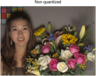  Picture rendering with original filter bank
• 
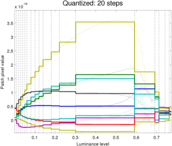  Filter coefficients of 20 levels QUANTIZED filter bank
• 
  Picture rendering with 20 levels QUANTIZED filter bank
• 
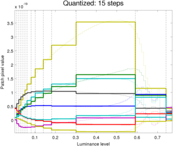  Filter coefficients of 15 levels QUANTIZED filter bank
• 
  Picture rendering with 15 levels QUANTIZED filter bank
• 
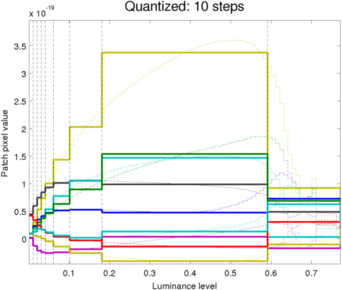  Filter coefficients of 10 levels QUANTIZED filter bank
• 
  Picture rendering with 10 levels QUANTIZED filter bank
• 
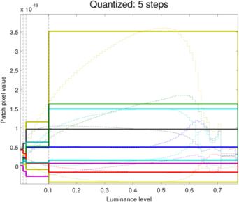  Filter coefficients of 5 levels QUANTIZED filter bank
• 
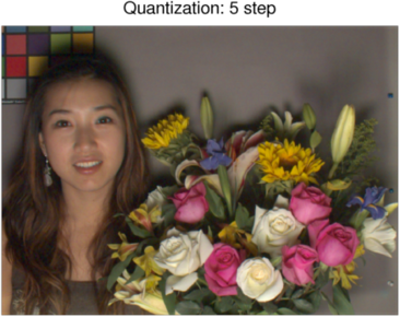  Picture rendering with 5 levels QUANTIZED filter bank

In our experiments, the amount of quantization was dropped further from 20 to 5 in steps of 5. The results are interesting; the picture from 5 quantized levels as seen above is almost indistinguishable from the that of 20 levels while since no saturation is observed, our quantized filters are almost exclusively used to render the picture (This algorithm was only implemented for the "no saturation" filters coefficients; the remaining portion of the filter bank retains the original quantized levels). The most distortion in the picture appears actually in the dark areas where the amount of noise increases slightly as we reduce the number of quantization bands.

In addition, the qualitative results of this procedure match the assumption in [1] that the rapid SNR changes in the lower response levels requires more densely sampled in that region. One benefit of this approach is that different levels of quantization can be accurately compared to choose the optimal numbers of levels depending on the application or product.

Conclusions and Future Work

In this project, we have explored different ideas aiming at reducing the storage requirement associated with the L3 filter structure.

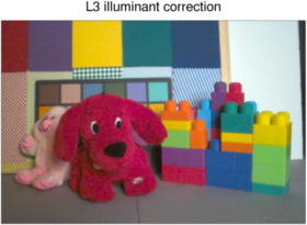
• Illuminant correction: We have looked at 3 different possible transformation aiming at removing the necessity to store an entire filter bank in order to perform illuminant correction in the case of an illuminant which would not be the reference one (D65 in our case). The 3 cases proved to be very promising, reducing the storage need of illuminant correction to less than 10 matrix coefficients without affecting too much the compensation of the illuminant.

• Luminance compression: The quasi-linear relationship between filters at neighboring luminance levels allowed us to compress (>50%) the number of coefficients necessary to store the L3 filters for a given illuminant without introducing a noticeable distortion.

• Luminance quantization: Our test on a densely sampled filter bank (along the luminance axis) seem to confirm the necessity to learn more filters for low luminance levels, while averaging filters can be learned for high luminance. Though preliminary, our results are a promising step towards the derivation of a quasi-optimal sampling of the luminance axis for traning purposes, reducing both the training duration and the storage requirement of the L3 filter bank.

From our results, we think that the following points could be addressed in order to further improve our understanding of the L3 filter structure and either increase compression or reduce the distortion resulting from one of the methods outlined here:

• Further improve illuminant correction transforms: Though promising, we have seen some limits to approximating the illuminant correction by linear transforms. In particular, we have not yet a complete understanding of how to deal with redundant color mosaics such as RGBW where the correctness of some of the linear relationships we assumed seemed weaker .

• Include more types of sensor CFA: It would be interesting to see how our findings extend to other types of CFA (CYMK,...)

• Improve the treatment of the saturated cases in illuminant correction": The L3 filters for saturated pixels do not seem to generally follow the linear relationship observed for the non-saturated cases. It would be interesting to find out if a good approximation can be used to integrate those cases into our illuminant correction methods.

• Include saturated cases in quantization study: In the time frame of this project, it was not possible for us to address the question of the luminance quantization in the case of filters with saturated pixels, because of the structure of the L3 filters. Adding them into our approach is a necessary step towards a general quantization solution for the L3 filter banks.

• Derive an optimal "universal' luminance quantization scheme: Starting from our preliminary result, finding such scheme would be a great improvement to the L3 framework, both in quality (lowered distortion) and practicality (training time/storage).

Overall, a lot can be done regarding the design choices of the L3 algorithm, as it is not always clear why the filters behave the way they do, and if different choices would not lead to results with the same quality, but with much reduced structural complexity. For example, the large variations of the filters observed for very high luminance could be artifact of the training process, while prolonging the smooth trend of the filters in the previous luminance bands might still give acceptable results. The fact that the relationship between changes in the filters, and the distortion observed on the rendered image will require a more extended study of the subjects that were touched in this project.

References _ List

[1] Tian, Lansel, Farrell and Wandell. Automating the design of image processing pipelines for novel color filter arrays: Local, Linear, Learned (L3) method. https://drive.google.com/file/d/0B0Gw85qGqJxhbXJlcmZjbmhOQ2s/edit?usp=sharing

[2] Wandell. "Color" In Foundations of Vision

Appendix I

All the code requires the L3 source code and the ISET camera code in order to render images. However, the processing of the L3 filter banks without rendering should generally not require them.

"scene" and "camera" are standard object structures from ISET and L3. In addition, the camera object is used to store the transform presented in this project. In general, L3 rendering requires to load scenes in a multispectral format.

Source code for illuminant correction: File:IlluminantCorrection.zip

Source code for compression across luminance levels File:CompressionAcrossLuminanceLevels.zip

Source code for luminance levels quantization File:LuminanceQuantization.zip

Appendix II

François:

Illuminance correction (code + wiki + slides)

Luminance quantization (code + slides)

Iretiayo:

Luminance compression (code + wiki + slides)

Luminance quantization (code + wiki)