Andy Lin
Introduction
It is extremely useful to render 3D scenes and be able to feed the radiance information of these scenes into camera simulation software such as ISET [2][4]. Synthesizing scenes allows for the control over scene attributes that could be difficult to obtain when working with real world scenes. For example, scene synthesis allows for the control over foreground objects, backgrounds, texture, and lighting. Most importantly, the depth information is very easy to obtain, in contrast to the complicated depth estimation algorithms for real-world scenes.
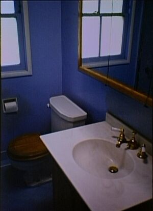
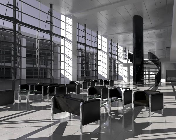
Often times, people criticize synthesized scenes and say that they are not realistic enough. However, with enough effort and precision, highly realistic scenes can be generated. See Figure 1 for examples of synthesized scenes with the Radiance software[6].
Figure 1: Rendered scenes can be quite realistic. These scenes, in particular, are example scenes from Radiance.
Moreover, if these rendered scenes can be fed into a camera simulation software such as ISET, then we could simulate photographs of these artificial scenes. Moreover, the additional 3D information allows for renderings of advanced photography attributes that have not been simulated extensively before in a well-controlled synthesized environment. For example, the 3D information allows for the simulation of multiple camera systems, proper lens depth-of-field simulation, synthetic aperture, flutter shutter, and even light-fields cameras.
For this project, I used the RenderToolBox software tool, provided by David Brainard[1] to synthesize example 3D scenes. The radiance of these scenes, along with the depth map were then fed into the ISET simulation environment for a simulated camera capture of the scene.
Methods
In order to use RenderToolBox, a deeper understanding of its architecture is required. RenderToolBox is actually a wrapper software tool of several other simulation software. In particular, Radiance, PsychToolBox, Physicalled Based Rendering (PBRT), and SimToolBox are used to help render an artificial scene. The most important software tool that RenderToolBox is built on, is Radiance, which is a scene rendering tool which contains a ray tracer.
RenderToolBox
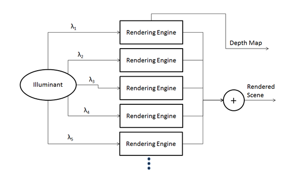
RenderToolBox works by repeatedly calling another a separate rendering engine. There are several rendering engines available in RenderToolBox such as Radiance and PBRT. Although these rendering engines are very capable, they are limited in their output. Most importantly, these rendering engines can only output images with a tri-chromatic colorspace. However, for proper camera simulation, we require multi-spectral data. This problem is the one that RenderToolBox addresses. In order to allow for multi-spectral renderings, it provides multiple input light sources to the rendering engine, each at a specific wavelength. The intensities of these monochromatic input light sources are at the corresponding intensities of the desired light sources of that wavelength. After the rendering engine renders these scenes with different wavelength light sources, it then combines the data obtained. RenderToolBox also allows for us to obtain a depth map of the scene, at the specified camera position. See Figure 2 for the data flow of RenderToolBox.
Figure 2: Data flow for RenderToolBox and interaction with rendering engine.
Available Objects To Render
A multitude of shapes, textures, lights, etc. can be rendered with Radiance, and therefore, with RenderToolBox as well. For example, Radiance is able to render different 3D shapes such as cones, spheres, cylinders, and cups. All these objects can then be made of different materials such as plastics, metals, and textures. Interesting lighting effects can be rendered as well for the scene. Not only can there be multiple light sources, but Radiance can also render glowing surfaces, mirrors, prisms, glass, and even mist. Also, any combination of different materials and lighting can be assigned to the objects.
Moreover, RenderToolBox and Radiance are able to use triangular meshes to create objects. This is a very powerful feature because any arbitrary object, which can be approximated with a 3D mesh can be rendered. In fact, RenderToolBox allows for the import of 3D meshes from 3D modeling software such as Maya.
Rendering Options
RenderToolBox is also highly customizable in terms of rendering options. There is access to different rendering engines to use (usually Radiance, or PBRT), as well as the camera angle, position, and field of view. The prominent light source can also be changed as well as the number of rendered light bounces. In other words, if there are highly reflective surfaces that can result in multiple light bounces, then the user can choose the number of light bounces that will be simulated when rendering.
Interface With ISET
Rendering multi-spectral scenes is useful, but being able to render these scenes in a camera simulation framework such as ISET could be even more useful. Interfacing with ISET is relatively straightforward. The output from RenderToolBox is a Matlab .mat file, which contains a cell array, with each cell specifying the radiance of the scene at every point in space. This cell array was then converted to a 3D matrix, with the 3rd dimension specifying wavelength, and the first 2 dimensions specifying radiance in the camera plane. This 3D matrix is then fed into an ISET scene. The proper light source and brightness is also specified for the ISET scene. See the Appendix for this code.
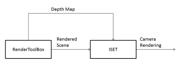
The second output from RenderToolBox is a depth-map. The depth-map is obtained by adding a rendering call to Radiance by modifying a RenderToolBox function. Although Radiance offers an output file for the depth-map, it is in a raw binary format. A Matlab script was written in order to properly read this data. After reading the depth map data, some data conditioning was performed to make sure that the depth data was within a proper range. See the Appendix for the code for this Matlab script. See Figure 3 for a block diagram of how RenderToolBox can interface with ISET.
Figure 3: RenderToolBox and ISET can interface with each other quite easily.
Simulating Lens Depth-of-Field Blur
One possible simulation using RenderToolBox data in ISET is lens depth-of-field(DOF) blur. A lens is able to converge light rays that originate from 1 point in space, back onto 1 point at the image plane. However, the point in space in which this lens can re-converge light is limited in distance from a lens. If the object distance is too close, the lens will not be strong enough to re-converge the light, resulting in a blurry circle corresponding to that one point in space. On the other hand, if the object distance is too far, the lens will be too strong, and the light rays will cross each other, then form a blurry circle, once again at the image plane. See Figure 4 for an illustration of this concept. Therefore, the Point Spread Function(PSF), or impulse response, for the lens will vary according to the depth of an object. For areas of the image which are at the focal plane, the PSF will be close to an impulse. For areas of the image which are further from the focal plane, the PSF will become an increasingly large circle, producing blur for areas of the scene which are not in focus.
Another parameter that can influence the blur amount of the PSF, given a fixed sensor plane, is the aperture of the lens. When the aperture of a camera is more open, light near the edges of the lens will be bent and redirected to a greater degree in order to converge light rays when an object is in focus. When an object is out of focus, due to geometry, light that hits areas further from the center of the lens will again be bent more, producing a larger blur circle, than if the aperture were smaller. In order to characterize lens blur, given an object distance and aperture size, Hopkins[3] defined the w20 parameter.
The W20 parameter
As described earlier, there are 2 different parameters that influence lens blur, given a fixed sensor plane, the object distance as well as the aperture size. The larger the aperture, the larger the DOF blur. The further the object is from the focal plane, the larger the DOF blur. The W20 parameters takes these 2 factors into account, and becomes a parameter for lens blur, which can then be used to calculate the optical transfer function (OTF), the Fourier transform of the PSF[3].
The W20 parameter is roughly derived as follows. First, we define the following pupil function, which predicts the response of the system to a single ray of light:

The imaginary term accounts for the phase shift that the lens introduces, which bends the light towards the center. The w20 function then describes the attenuation that the lens introduces, as a function of the distance from the center of the lens. Note that x and y are coordinates in the plane of the lens. In other words, if one is to look through the lens from the front, they would be looking at the x-y plane directly. In this expression, w20 is a function of x and y, so the w20 parameter varies with x and y, which makes sense since the attenuation of the lens varies depending on the distance from the center of the lens, which usually has the least attenuation of light.
According to Fourier optics, the resulting electric field F at the sensor plane is found by taking the Fourier transform as follows:

The perceived intensity of the image is then the magnitude of the resulting electric field, squared.

This result is similar to the simpler Young's Double-slit Experiment, where the intensity of light at the image plane is the magnitude of the Fourier Transform of the indicator function which indicates the pattern of the slits[7]. Since this perceived intensity is that of the response to a single point source of light, this intensity is referred to as the PSF.
The OTF that we wish to calculate is actually the Fourier Transform of the PSF.

where g represents the OTF. Using Parseval's Theorem, we can then rewrite the OTF as follows:

Next, we perform a simple change of variables to obtain the following expression:

Finally, we rewrite g as a function of s only, by setting t to 0 by accounting for the circular symmetry of the expression. D(s) then becomes the 1D OTF, which can be expanded to a 2D OTF by considering symmetry. Note that D(s) is a function of a, which is a function of w20.

The region of integration for D then becomes the intersection of 2 circles, as described in Figure 5, due to the two shifted pupil functions, f, which are radially symmetric.
The simplification of this integral then becomes the following expression, which can written as the weighted sum of various Bessel functions:

Figure 5: The area of integration includes the intersection of the two circles.
Simulating Lens Blur
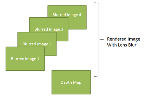
Once the w20 parameter is found, we can then simulate lens blur by employing the following method. Since the lens blur must be feasible, we bin the object distances uniformly. Since we assume that the aperture of the lens will not change, for different objects, which is a reasonable assumption, the only attribute of the system that modifies the w20 parameter, is object distance. Thus, for every discrete distance, we calculate the corresponding w20 parameter, then calculate the OTF, given this w20 parameter, and obtain a blurred image corresponding to that specific depth. Next, given the depth-map, we can combine the different blurred images, by using the correct blurred image for a specific depth. See Figure 6 for an illustration of this concept.
I attempted to simulate this lens blur, with the previously described algorithm in ISET. However, the implementation is not yet feasible, since one of the ISET functions, defocusMTF, takes a very long time to run. This issue should be looked at in detail in the future, to allow for an ISET simulation of DOF lens blur.
Figure 6: The use of different blurred images, each with the blur corresponding to a different depth, and a depth map can be used to render an image with lens blur.
Results
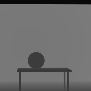
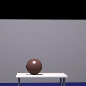
I was able to successfully render a basic scene, which is composed of a table with a sphere on top of it, within a rectangular indoor room. D65 was used as the illuminant, and all surfaces are glossy. The simulated camera was placed approximately directly in front of the table. See Figure 7 for an example monitor render of this scene. This rendering was taken directly from RenderToolBox. See Figure 8 for the successful depth-map rendering of the same table-sphere scene.
After rendering the table-sphere scene in RenderToolBox, the radiance values were imported into ISET, along with the illuminant, D65. Afterwards, this scene was then fed into a standard camera image processing pipeline in ISET. See Figure 9 for the ISET rendering of the table-sphere scene. Although the ISET rendering for DOF lens blur is not completed, renderings of this type of image was produced in Photoshop, as inspiration for what is possible with depth information and rendering data. See Figure 10 for examples of these results with various blur amounts, and focal points.
Figure 7: A monitor rendering of the table-sphere scene.
Figure 8: Depth-map of the table-sphere scene. Darker areas signify closer depth, while lighter areas signify further depth.
Figure 9: ISET rendering of table-sphere.
Figure 10: ISET rendering of table-sphere, with Photoshop depth blurring, at various focal points, and aperture sizes.
Discussion
As illustrated, I was able to render an example scene in RenderToolBox, render a depth-map, and feed this data into ISET. However, this is only the first step of this simulation process. Many more different types of renderings are possible. First, a proper DOF lens blur rendering must be achieved in ISET. Although the Photoshop renderings look visually appealing, there is little control over the blurring operation. Simulation in ISET would be much more scientifically correct, and also convenient for research purposes.
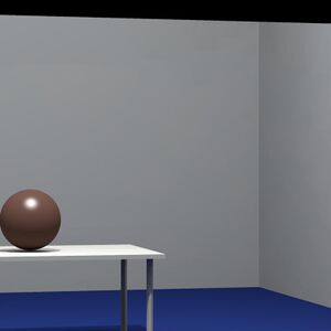
Moreover, after proper integration into ISET, further simulations can be performed. For example, synthetic apertures, light-fields, and even multiple-camera systems can be simulated. As an inspiration, see Figure 11 for an example multiple-camera set of renderings. These multiple camera system simulations are particularly useful for binocular camera system simulation. Even expensive camera arrays can be simulated and analyzed easily without the tedious and costly setup of a true camera array. Another topic to explore is view-point synthesis. Since we can produce practically arbitrary view-points with cameras, the accuracy of view-point synthesis algorithms such as the one described in [5] can be explored. Since we have access to the ground truth images, more accurate algorithm performance assessment can be achieved. Although the camera view-point and orientation can be placed almost arbitrarily, issues with rendering arise if the view-point is too extreme.
Figure 10: Example multiple-camera rendering.
Conclusion
As illustrated, we were able to create an example scene in RenderToolBox, and feed the radiance data and depth-map into ISET. Although we could not properly render a DOF blurred image, such a task is feasible and will be completed in the near future. Different experimentation with view-point variation, and the ability to simulate different apertures allows for future renderings of synthetic apertures, multiple-camera systems, and even light-field cameras. Moreover, more complex scenes could be rendered in the future, with the help of perhaps Maya, a 3D prototyping software. Synthetic renderings of multi-spectral scenes with RenderToolBox seems promising and will be pursued further in the future. Perhaps more novel scenes, such as those featuring different textures, glass surfaces, objects with specularity, or mixtures of materials, would provide for interesting results. Nevertheless, this initial study shows that the synthesis of artificial scenes with RenderToolBox, which can then be used as 3D scenes for ISET, is quite useful, and can open the doors to many interesting subsequent camera simulations.
References
[1] D. Brainard, C. Broussard, RenderToolBox Paper (To Be Published).
[2] J. E. Farrell, F. Xiao, P. Catrysse, and B. Wandell, "A simulation tool for evaluating digital camera image quality," In Proc. SPIE Int. Soc. Opt. Eng., Vol. 5294, 124, 2004.
[3] H. H. Hopkins. "The frequency response of a defocused optical system," Proceedings of the Royal Society of London, Series A, Mathematical and Physical Sciences, Vol. 231, 1184, 1955.
[4] P. Y. Maeda. P. B. Catrysse and B. A. Wandell, "Integrating lens design with digital camera simulation," In Proc. SPIE Int. Soc. Opt. Eng., Vol. 5678, 48, 2005.
[5] J Ohm, M. E. Izquierdo, "Circuits and Systems, "An object-based system for stereoscopic viewpoint synthesis", Circuits and Systems for Video Technology, IEEE Transactions on , Vol. 7, 5, 1997.
[6] G. J. Ward, F. M. Rubinstein, and R.D. Clear, "A Ray Tracing Solution for Diffuse Interreflection", SIGGRAPH, Vol. 22, 4, 1988.
[7] T. Young, "The Bakerian Lecture: Experiments and Calculations Relative to Physical Optics." Philosophical Transactions of the Royal Society of London Vol. 94, 1804.
Acknowledgements
Special thanks to Professor Brian Wandell, Joyce Farrell, and Steve Lansel for the advise and help for this project and Psych 221 in general. Also, I'd like to thank David Brainard, Michael Perry, and Bob Dougherty for the help in setting up RenderToolBox.
Appendix
Depth-Map Generation Code
%condition the data, throw away garbage
A2 = A .* (abs(A) < 1000);
A2 = A2 (1:test^2);
%reshape data
A3 = reshape(A2, [test test]);
%make the range shown appropriate
% lowerLimit = 900;
% upperLimit = 1000;
% viewImage = abs(A3 - 900)/100;
% viewImage = abs(A3 - lowerLimit)/(upperLimit-lowerLimit);
viewImage = abs((A3 - lowerLimit)/(upperLimit-lowerLimit));
viewImage= viewImage';
figure; imshow(viewImage);
imwrite(viewImage, 'depthMapView.tif');
ISET Integration Code (edit to view correctly)
%% SimulateSystemDataFlow
% **heavily based off of the included ISET script: s_SimulateSystem.m
% This script introduces how to create the full array of elements that make % up the image simulation steps. The script begins by creating a full % spectral scene. The radiance data are passed through the optics to create % an irradiance image at the sensor surface. The irradiance is then % captured by a simulated sensor, resulting in an array of output voltages. % % To learn more about a particular function, type "help function" as in % "help sensorCreate". There are also online descriptions of the functions % at http://www.imageval.com/public/Products/ISET/Manual/ISET_Functions.htm % % Copyright ImagEval Consultants, LLC, 2010.
%% Init % We will use this wavelength, which is a bit odd, just to illustrate that % we can read everything at the correct wavelengths
wave = 400:5:700;
% It is also possible to expand the range to include wavelengths in the near infrared range
% In this case one should use scene data (see below) that has spectral energy over this
% range. For example:
% patchSize = 8;
% spectrum.wave = (380:4:1068)';
% scene = sceneCreate('macbethEE_IR',patchSize,spectrum);
%% SCENE % % There are several ways to create a scene. One is to use the sceneCreate % function. Two examples are listed here. For a complete list type "help sceneCreate" % % scene = sceneCreate('slantedEdge'); % scene = sceneCreate('macbeth',32);
%One advantage of using synthetic scenes is that they are noise free. The %multispectral images have noise that is generated from the multispectral %camera system. % scene = sceneFromFile('scene_orange_rad.mat', 'multispectral'); % load 'scene_orange_rad.mat'; makeRadianceScene
% Each scene has a stored illuminant. % Below we show how to change the scene illuminant % curIlluminant = sceneGet(scene,'illuminantdata'); % newIlluminant = blackbody(wave,666); % scene = sceneSPDScale(scene,curIlluminant,'divide'); % scene = sceneSPDScale(scene,newIlluminant,'multiply');
% A second method for creating a scene is to read data from a file. % ISET includes a few multispectral scenes as part of the distribution. % These can be found in the data/image/multispectral directory. % fullFileName = ... % fullfile(isetRootPath,'data','images','multispectral','StuffedAnimals_tungsten-hdrs.mat'); % scene = sceneFromFile(fullFileName,'multispectral');
% You can also select the file (or many other files) using the command: % % fullFileName = vcSelectImage; % % and navigating to the proper directory and file that contains the scene % data. ISET will interpolate RGB files (such as JPEG files). The % spectral information that it creates, however, is not accurate.
% Once the scene is loaded, you can adjust different properties % using the sceneSet command. Here we adjust the scene mean luminance and % field of view. scene = sceneAdjustLuminance(scene,200); % Candelas/m2 scene = sceneSet(scene,'fov',26.5); % Set the scene horizontal field of view scene = sceneInterpolateW(scene,wave,1); % Resample, preserve luminance
% It is often useful to visualize the data in the scene window vcAddAndSelectObject('scene',scene); sceneWindow;
% When the window appears, you can scale the window size and adjust the % font size as well (Edit | Change Font Size). There are many other options % in the pull down menus for cropping, transposing, and measuring scene % properties. % %% OPTICS % % The next step in the system simulation is to specify the optical image % formation process. The optical image is an important structure, like the % scene structure. We adjust the properties of optical image formation % using the oiSet and oiGet routines. % % The optical image structure contains the irradiance data and a % specification of the optics. The optics itself is so complex that we % have created a special optics structure as well that can be manipulated % by opticsGet and opticsSet commands. % % ISET has several optics models that you can experiment with. These % include shift-invariant optics, in which there is a different % shift-invariant pointspread function for each wavelength, and a ray-trace % method, in which we read in data from Zemax and create a shift-variant % set of pointspread functions along with a geometric distortion function. % % The simplest is method of creating an optical image is to use % the diffraction-limited lens model. To create a diffraction-limited % optics with an f# of 4, you can call these functions
oi = oiCreate; optics = oiGet(oi,'optics'); optics = opticsSet(optics,'fnumber',4); %.5 to allow for shallow DOF % optics = opticsSet(optics, 'nWave', 31); %number of waves...might need a better way of doing this later
% In this example we set the properties of the optics to include cos4th
% falloff for the off axis vignetting of the imaging lens, and we set the
% lens focal length to 3 mm.
optics = opticsSet(optics,'offaxis','cos4th');
optics = opticsSet(optics,'focallength',2.4e-3); % from lens calibration software
% Many other properties can be set as well (type help opticsSet or doc % opticsSet).
% We then replace the new optics variable into the optical image structure. oi = oiSet(oi,'optics',optics);
% % We use the scene structure and the optical image structure to update the % % irradiance. oi = oiCompute(scene,oi); % we may need to disable some of the blurring here to make way for a % clearer image - may need to integrate with this function later
% % We save the optical image structure and bring up the optical image % % window. % vcAddAndSelectObject('oi',oi); oiWindow;
% %% apply defocus - should put this section into a single function or script
% %% later
%
% %do a linear sweep of distance
% fLength = opticsGet(optics,'focal length','m');
% D0 = opticsGet(optics,'power');
%
% nSteps = 500;
% % objDist = linspace(fLength*1.5,100*fLength,nSteps);
% objDist = linspace(fLength*1.5,200*fLength,nSteps);
% D = opticsDepthDefocus(objDist,optics); %compute defocus in terms of amount of power needed to put object in focus
%
% %visualize
% % vcNewGraphWin
% % semilogx(objDist/fLength,D/D0);
% % title('Sensor at focal length')
% % xlabel('Distance to object (units: focal length)');
% % ylabel('Relative dioptric error')
% % grid on
% % t = sprintf('Focal length %.1f (mm)',fLength*ieUnitScaleFactor('mm'));
% % legend(t)
%
% % Defocus with respect to image plane different from focal image plane
%
% % In this example, we arrange the distance between the lens and sensor to
% % be a little longer than the focal length. In this case objects in good
% % focus are closer than infinity. We calculate the in-focus plane in both
% % meters and focal lengths.
% s = 1.1;
% D = opticsDepthDefocus(objDist,optics,s*fLength);
% [v,ii] = min(abs(D));
%
% fprintf('Sensor plane is located %.3f focal lengths behind thin lens.\n',s)
% fprintf('In focus object distance (m) from thin lens: %.3f.\n',objDist(ii));
% fprintf('In focus object is %.3f focal lengths from thin lens.\n',objDist(ii)/fLength);
%
% % The dioptric error as a function of object distance (in units of focal
% % length
% vcNewGraphWin;
% semilogx(objDist/fLength,D);
% xlabel('Object distance (focal lengths)');
% ylabel('Dioptric error (1/m)')
% grid on
% t = sprintf('Focal length %.1f (mm)',fLength*ieUnitScaleFactor('mm'));
% legend(t)
%
%
% % The dioptric error depends on the object distance. The impact this
% % will have on defocus depends on the pupil aperture.
% p = opticsGet(optics,'pupil radius');
%
% % The w20 parameter is used by Hopkins to predict the amount of defocus.
% % Notice that the formula depends on both the relative defocus (D and D0)
% % and the pupil size.
% s = [0.5 1.5 3];
% leg = cell(1,length(s));
% w20 = zeros(length(D),length(s));
% lType = {'k-','r--','b--','g-'};
% vcNewGraphWin;
% for ii=1:length(s)
% w20(:,ii) = (s(ii)*p)^2/2*(D0.*D)./(D0+D); % See human Core
% semilogx(objDist/fLength,w20(:,ii),lType{ii}); hold on;
% leg{ii} = sprintf('%.2f (mm)',p*s(ii)*ieUnitScaleFactor('mm'));
% end
% hold off; grid on; legend(leg)
% title('Depth of field')
% xlabel('Object distance (re: focal length)');
% ylabel('Hopkins w20 (defocus)');
%
%
% %here we will assume a pupil size of 3*p to get the most defocus
% %we will use distance increments of 25 so that there aren't too many
% %different images to blur and the computation won't take too long
% newOi = oi;
% prevObjDist = 0;
%
% for count = 1:25:length(objDist)
% display(count)
% %compute OTF given defocus amount
% %frequencySupport = ?
% frequencySupport(:,:,1) = zeros(size(scene.data));
% frequencySupport(:,:,2) = ones(size(scene.data)) * 1000;
% % not sure what the frequency support should be, will guess a large range for now
%
% %find OTF for every distance, given the w20 parameter
% OTF = defocusMTF(optics,frequencySupport,w20(count,3));
%
% %apply OTF on optical image
% tempOi = oiApplyOTFDefocus(oi,scene, OTF)
%
% %2 choices
% %1)save optical image in a cell element (hopefully this doesn't make it
% %run out of memory...)
% %2)save only the relevant part of optical image(the part that is within
% %the correct depth, into one optical image) to save space
% %we will try choice #2 for now... may need to modify for later
%
% % newOi
%
%
% depthIndicator = (scene.depthMap >= prevObjDist) .* (scene.depthMap < objDist(count));
%
% newOi.data.photons(depthIndicator>0) = tempOi(depthIndicator>0);
% prevObjDist = objDist(count);
% end
%
% oi = newOi;
%%
% From the window you can see a wide range of options. These include % insertion of a birefringent anti-aliasing filter, turning off cos4th % image fall-off, adjusting the lens properties, and so forth. % % You can read more about the optics models by typing "doc opticsGet". % You can see an online video about using the ray trace software at: % http://www.imageval.com/public/Products/ISET/ApplicationNotes/ZemaxTutorial.htm % %% SENSOR % % There are a very large number of sensor parameters. Here we illustrate % the process of creating a simple Bayer-gbrg sensor and setting a few of % its basic properties. % % To create the sensor structure, we call sensor = sensorCreate('bayer-gbrg');
% We set the sensor properties using sensorSet and sensorGet routines. % % Just as the optical irradiance gives a special status to the optics, the % sensor gives a special status to the pixel. In this section we define % the key pixel and sensor properties, and we then put the sensor and pixel % back together.
% To get the pixel structure from the sensor we use: pixel = sensorGet(sensor,'pixel');
% Here are some of the key pixel properties voltageSwing = 1.15; % Volts wellCapacity = 9000; % Electrons conversiongain = voltageSwing/wellCapacity; fillfactor = 0.45; % A fraction of the pixel area pixelSize = 2.2*1e-6; % Meters darkvoltage = 1e-005; % Volts/sec readnoise = 0.00096; % Volts
% We set these properties here pixel = pixelSet(pixel,'size',[pixelSize pixelSize]); pixel = pixelSet(pixel,'conversiongain', conversiongain); pixel = pixelSet(pixel,'voltageswing',voltageSwing); pixel = pixelSet(pixel,'darkvoltage',darkvoltage) ; pixel = pixelSet(pixel,'readnoisevolts',readnoise);
% Now we set some general sensor properties exposureDuration = 0.030; % Seconds dsnu = 0.0010; % Volts prnu = 0.2218; % Percent (ranging between 0 and 100) analogGain = 1; % Used to adjust ISO speed analogOffset = 0; % Used to account for sensor black level rows = 466; % number of pixels in a row cols = 466; % number of pixels in a column
% Set these sensor properties sensor = sensorSet(sensor,'exposuretime',exposureDuration); sensor = sensorSet(sensor,'rows',rows); sensor = sensorSet(sensor,'cols',cols); sensor = sensorSet(sensor,'dsnulevel',dsnu); sensor = sensorSet(sensor,'prnulevel',prnu); sensor = sensorSet(sensor,'analogGain',analogGain); sensor = sensorSet(sensor,'analogOffset',analogOffset);
% Stuff the pixel back into the sensor structure sensor = sensorSet(sensor,'pixel',pixel); sensor = pixelCenterFillPD(sensor,fillfactor);
% It is also possible to replace the spectral quantum efficiency curves of % the sensor with those from a calibrated camera. We include the % calibration data from a very nice Nikon D100 camera as part of ISET. % To load those data we first determine the wavelength samples for this sensor. wave = sensorGet(sensor,'wave');
% Then we load the calibration data and attach them to the sensor structure fullFileName = fullfile(isetRootPath,'data','sensor','NikonD100.mat'); [data,filterNames] = ieReadColorFilter(wave,fullFileName); sensor = sensorSet(sensor,'filterspectra',data); sensor = sensorSet(sensor,'filternames',filterNames); sensor = sensorSet(sensor,'Name','Camera-Simulation');
% We are now ready to compute the sensor image sensor = sensorCompute(sensor,oi);
% We can view sensor image in the GUI. Note that the image that comes up % shows the color of each pixel in the sensor mosaic. Also, please be aware % that % * The Matlab rendering algorithm often introduces unwanted artifacts % into the display window. You can resize the window to eliminate these. % * You can also set the display gamma function to brighten the appearance % in the edit box at the lower left of the window. vcAddAndSelectObject('sensor',sensor); sensorImageWindow;
% There are a variety of ways to quantify these data in the pulldown menus. % Also, you can view the individual pixel data either by zooming on the % image (Edit | Zoom) or by bringing the image viewer tool (Edit | Viewer). % % Type 'help iexL2ColorFilter' to find out how to convert data from an % Excel Spread Sheet to an ISET color filter file or a spectral file/ % % ISET includes a wide array of options for selecting color filters, % fill-factors, infrared blocking filters, adjusting pixel properties, % color filter array patterns, and exposure modes. %% Image Processor % % The image processing pipeline is managed by the fourth principal ISET % structure, the virtual camera image (vci). This structure allows the % user to set a variety of image processing methods, including demosaicking % and color balancing. vci = vcImageCreate;
% The routines for setting and getting image processing parameters are % imageGet and imageSet. % vci = imageSet(vci,'name','Unbalanced'); vci = imageSet(vci,'scaledisplay',1); vci = imageSet(vci,'renderGamma',0.6);
% The default properties use bilinear demosaicking, no color conversion or % balancing. The sensor RGB values are simply set to the display RGB % values. vci = vcimageCompute(vci,sensor);
% As in the other cases, we can bring up a window to view the processed % data, this time a full RGB image. vcAddAndSelectObject(vci); vcimageWindow
% You can experiment by changing the processing parameters in many ways, % such as: vci2 = imageSet(vci,'name','More Balanced') vci2 = imageSet(vci2,'internalCS','XYZ'); vci2 = imageSet(vci2,'colorConversionMethod','MCC Optimized'); vci2 = imageSet(vci2,'colorBalanceMethod','Gray World');
% With these parameters, the colors will appear to be more accurate vci2 = vcimageCompute(vci2,sensor);
vcAddAndSelectObject(vci2); vcimageWindow
% Again, this window offers the opportunity to perform many parameter % changes and to evaluate certain metric properties of the current system. % Try the pulldown menu item (Analyze | Create Slanted Bar) and then run % the pulldown menu (Analyze | ISO12233) to obtain a spatial frequency % response function for the slanted bar image in the ISO standard. %
%% END
