Benbrook Chen Leckie Lopez

Introduction
Image alignment is the process of matching one image called template with another image. It is also referred to as image registration. It is a crucial step in many image systems engineering applications such as video stabilization, summarization, and the creation of panoramic mosaics. It has a broad variety of applications such as computer vision, medical imaging, and military automatic target recognition.
Background
Previous work on image alignment algorithms fall into two categories: intensity-based and feature-based. Intensity-based algorithms compare the spatial intensity in sets of images, while feature-based algorithms detect image features like objects or lines. Image alignment algorithms can alternatively be sorted according to the transformation on the target image space to the reference image space. Some models use linear transformations, while other models use non-linear transformations that are elastic or non-rigid.
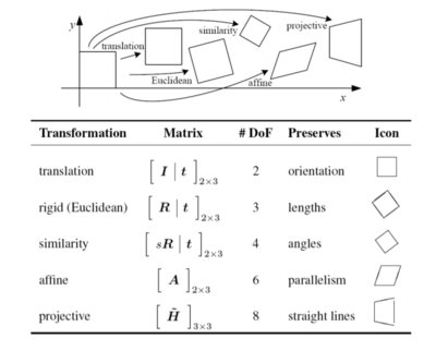
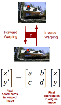
The first figure shows that two images with similar content can be realigned using different types of linear transformations. The second figure shows that when images become warped, they have undergone a transformation that changes their pixel space orientation. Image alignment can reverse this transformation. The image alignment can be represented with a linear transformation matrix.
Methods
The main goal of this project is to experiment with existing image alignment algorithms and analyze their performance. We will focus on comparing algorithms that utilize feature-based, linear transformation models. We used data from the ISET3D software on simulated images taken by various cameras and sensors, and images where the object is moving as well as the global scene. The image alignment algorithms will work with other image formats and types as well, such as iPhone images.
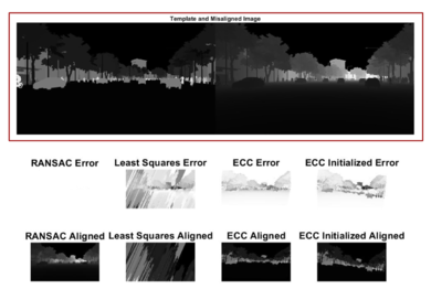
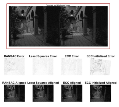
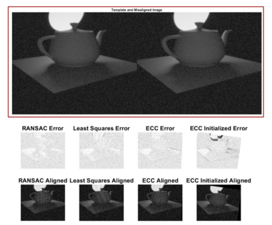
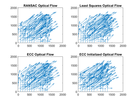
The alignment algorithms we tested rely on identifying a delta_x and delta_y for each pixel, that describe the difference in "identical" pixels between the image we want to align to, called the target image, and the image we are trying to align, called the warped image. The scripts provided provide plots showing the target and warped images, and then the error of each algorithm and the alignment results. Once we align images, we use mean squared error (MSE) and structural similarity index (SSIM) as metrics to compare the results between algorithms. The optical flow map for each algorithm is found to help visualize the delta_x and delta_y values (e.g. the apparent direction of alignment).
Images in black and white are described by 2D array (x by y by 1) of uint8 values in Matlab, where uint8 is an 8 bit integer between 0 and 255. Colored images are described by a 3D array (x by y by z) in Matlab, where each pixel has 3 associated uint8 values representing R,G, and B.
The scripts on this page request installation of the Computer Vision Toolbox from Mathworks, and the IAT toolbox which can be found here: https://sites.google.com/site/imagealignment/home
Algorithms
Speeded Up Robust Features (SURF)
Our first two algorithms are based on Speeded Up Robust Features (SURF), a patented feature detector and descriptor. SURF accomplishes the task of finding correspondences between two images of the same scene. It accomplishes this in three steps: (1) “interest points” are selected at distinctive locations in the image, (2) the neighborhood of every interest point is represented by a feature vector, and (3) the descriptor vectors are matched between the different images. It is important that the detector is repeatable so that it can reliably find the same interest points under different viewing conditions. It is also important for the descriptor to be distinctive so that it can be broken out from noise, errors, and deformations.
Random Sample Consensus (RANSAC)
RANSAC is a paradigm that fits a model to experimental data, and it is capable of interpreting and smoothing data containing errors, or outliers. This is ideal for interpreting data that comes from error-prone feature detectors, such as SURF. Unlike least squares, RANSAC is capable of smoothing data that contains a significant percentage of gross errors, which is common in scene analysis. Instead of using as much of the data as possible to obtain a solution, RANSAC uses a small initial data set and then enlarges it with consistent data. Once a set of mutually consistent points is identified, a smoothing technique such as least squares is used to compute an improved estimate. Using RANSAC requires choosing key parameters such as the number of data points, fitting threshold, and the inlier/outlier boundary. It excels in the terms of data variance, but it is subject to high processing times. Also, if there are too many outliers (approximately), it will break down and not be effective.
Least Squares
A classical technique for parameter estimation that optimizes a fit to all of the presented data. It does not detect and reject gross errors, or outliers. It relies on the assumption that the size of the dataset will be large enough that there will be enough good values to smooth out any gross deviations. The least squares method solves the image alignment problem by minimizing the sum of the squared residuals using a cost function. It is also possible to do weighted least squares, which defines how far the image is from the mean. The least squares method can be computationally costly depending on the matrix size.
Enhanced Correlation Coefficient (ECC)
ECC is an image alignment algorithm that achieves high accuracy in parameter estimation. It combines the low computation cost of gradient-based approaches with the performance of direct search techniques. Furthermore, it improves on the problem of brightness constancy. Since it considers the enhanced correlation coefficient, its performance remains unchanged in illumination changes and photometric distortions. The iterative scheme used for the optimization problem turns out to be linear, which reduces computational complexity.
The algorithm works by taking two unregistered images as inputs, the input image and the template image. It estimates the 2D geometric transformation, applies it to the input image, and then provides a warped image registered to the template image. This implementation compensates for larger displacements, but may need an initialization for larger displacements or strong geometric distortions, which can be accomplished by feature matching or a search scheme for coarse alignment.
Test Metrics
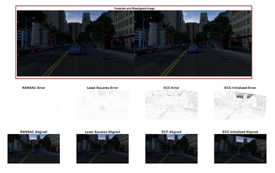
In order to test the results of our alignment algorithms, we used two different test metrics to evaluate our images. Figure 3 shows an example image with various test metrics results.

Mean Square Error (MSE)
MSE is a quantitative measure of signal quality. MSE is always a positive value that measures the quality of an estimator and values closest to zero are better. MSE is a simple to implement and is widely used to gauge error signal accuracy. It describes a physical quantity, which sit eh energy of the error signal. The MSE is convention in the field of signal processing, optimization, and image alignment. However, MSE is not well matched to the human perception of images. Therefore, its effectiveness as a judge of image alignment is limited.
MSE is computed by averaging the squared intensity differences of distorted and reference image pixels, but two distorted images with the same MSE may have very different types of errors, some of which are much more visible than others. Most perceptual image quality assessment approaches proposed in the literature attempt to weight different aspects of the error signal according to their visibility, as determined by psychophysical measurements in humans or physiological measurements in animals. Therefore, MSE is probably not the best metric for perceived alignment quality.
Structural Similarity Index (SSIM)
The SSIM quantifies the degradation of image quality after processing or losses during data transmission.The SSIM takes two images from the same image capture and measures the perceptual difference. SSIM was created as an improvement to other traditional methods like peak signal-to-noise ratio (PSNR) and mean squared error (MSE). SSIM is meant to predict the human perception of quality. Because of this, it only measures the perceptual difference, so the reference image must be of high quality. Therefore it is more suited to judge the quality of image alignment algorithms. Desired values are as close to 1 as possible (meaning the structural similarity is 100%).
While MSE and PSNR estimate absolute errors, SSIM calculates changes in structural information and takes into account image perception through luminescence masking and contrast masking components. Structural information is defined as the strong correlation between pixels that are spatially close. The correlations can elucidate structural information of the image scene, like objects. Luminance masking is the concept that distortions are more visible in darker regions. Contrast masking is the concept that distortions are less noticeable in areas of the image that are highly textured.
Optical Flow
Optical flow is the pattern of apparent motion of a visual scene. The optical flow can be calculated by finding the delta_x and delta_y of each pixel for two or more 2D image frames (voxels for 3D image frames) captured at different times, or from different angles. This method relies on differentiation since it uses the Taylor series approximations of the image signal. It can be useful to visualize the optical flow because in some cases of alignment, we only care about seeing which "direction" an image frame is moving.
Results
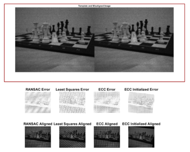
These are the 5 image pairs on which the 4 alignment algorithms were used.
 |
 |
 |
 |
 |
Conclusions
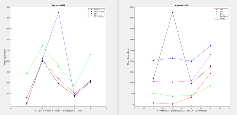
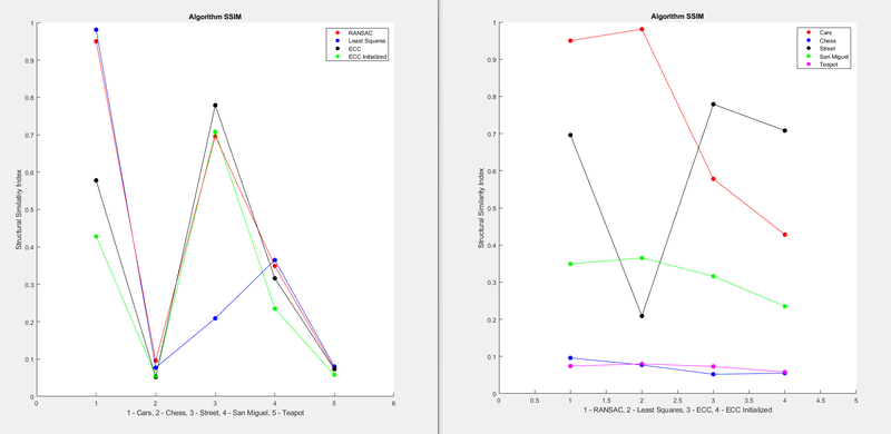
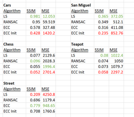
After running five sets of images through the four different algorithms, they were evaluated according to both test metrics, and the results are as follows:
As a reminder, SSIM values closest to 1 and MSE values closest to 0 indicate the best performance.
 |
 |
 |
 |
Our results showed excellent agreement between the SSIM and MSE test metrics. There was only one instance, in the chess image, where they did not select the same image as having the best performance. In every other case, they both agreed on the best and worst performers for each set of pictures.
Least squares proved to be the best algorithm in three of the picture sets, second place in another, and last place only once. ECC Initialized was generally the worst performer, but it was best for the street scene, which is the same one that the least squares performed worst in. The street scene pictures being different from the other 4 picture sets must have contributed to this result.
References
[1] Oleg Krivtsov, “Image Alignment Algorithms,” Code Project, 2008.
[2] Richard Szeliski (2007), "Image Alignment and Stitching: A Tutorial", Foundations and Trends® in Computer Graphics and Vision: Vol. 2: No. 1, pp 1-104.
[3] H.Bay, A.Ess, T.Tuytelaars, L.V.Gool, “SURF: Speeded Up Robust Features”, Computer Vision and Image Understanding (CVIU), Vol. 110, No. 3, pp. 346–359, 2008.
[4] Martin A. Fischler and Robert C. Bolles (June 1981). “Random Sample Consensus: A Paradigm for Model Fitting with Applications to Image Analysis and Automated Cartography”. Comm. of the ACM 24 (6): 381–395.
[5] G.D. Evangelidis, E.Z. Psarakis, Parametric Image Alignment using Enhanced Correlation Coefficient Maximization", IEEE Trans. on PAMI, vol. 30, no. 10, 2008.
[6] G.D. Evangelidis, “IAT: A Matlab toolbox for image alignment", https://sites.google.com/site/imagealignment/, 2013.
[7] Z. Wang and A. C. Bovik, "Mean squared error: Love it or leave it? A new look at Signal Fidelity Measures," in IEEE Signal Processing Magazine, vol. 26, no. 1, pp. 98-117, Jan. 2009. doi: 10.1109/MSP.2008.930649
[8] Z. Wang, A. C. Bovik, H. R. Sheikh and E. P. Simoncelli, “Image quality assessment: From error visibility to structural similarity,” IEEE Transactions on Image Processing, vol. 13, no. 4, pp. 600-612, Apr. 2004.
Appendix
Here is a .zip file containing our Matlab code and test images.
