Chris Baldassano

Identifying ROIs using SVM Performance

"Searchlight"-based approaches have become popular in fMRI data analysis. Rather than applying statistics to predefined regions of the brain, the entire brain volume can be searched for information related to the stimulus [1]. In this project, I use the performance of a Support Vector Machine as a measure of the information that a brain area contains about the presented stimulus. After discovering relevant ROIs, I also perform a complementary connectivity analysis to determine which regions contain different types of information about the stimulus.

Background

Scene Processing

The dataset being used for this project is designed to investigate natural scene perception (see Data Acquisition below). This research area has begun to attract significant attention, since humans display an incredible proficiency at classifying natural scenes: recognition can occur with presentation times as short as 100 ms [2] and subjects can access many details about scenes in only a glance [3]. This efficiency places constraints on the neural basis of scene perception, and suggests that modeling this process may be tractable.

Support Vector Machines

Support Vector Machines (SVMs) are designed to learn linear classifiers in high-dimensional spaces. By substituting the normal linear dot product with a modified kernel, it is also possible to learn classifiers in transformed feature spaces. In this project, I use the Radial Basis Function (RBF) and train the SVM using a variant of Sequential Minimal Optimization [4].

Complementary Connectivity

The connectivity analysis for this project was conducted based on the graphical model in [5], as shown in Figure 1. The probability estimates output from each SVM are the X variables. Rather than having each ROI "vote" independently to predict the scene type, the predictions from multiple ROIs are allowed to interact in the middle layer. If a connection between two of the Y variables improves classification performance, this indicates that the connected ROIs have complementary information about the scene. Connectivity is learned by comparing classification performance with all the Ys unconnected and with one pair of Ys connected. All of the pairwise connections that improve performance are then added to the final connectivity graph. Although this procedure is not guaranteed to find the minimal connectivity graph, it decreases the running time from $O(2^{n^{2}})$ to $O(n^{2})$.

Note that in order to evaluate the performance of a given graph structure, it is necessary to learn the edge weights of the graph. Unfortunately, there is no closed-form expression for this maximization, so iterative methods are required. Even more unfortunately, the objective function is not concave, so the edge weights we learn in an iterative algorithm may depend on the initial values with which we seed the algorithm. The approach taken in this case is to simply run gradient ascent with different starting values, and observe which graph structures frequently give good performance.

• 

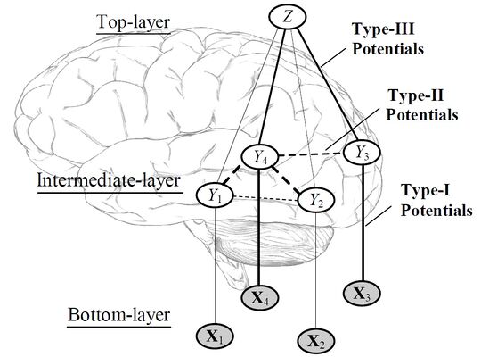  Figure 1

Methods

Data Acquisition

The data used is from the experiment described in [6]. Subjects passively viewed color images of six types of natural scenes: beaches, buildings, forests, highways, industry, and mountains. The stimuli were presented in a block design, with each block composed of 10 images from the same category displayed for 1.6 seconds each (8 brain acquisitions were made during each block). The subject viewed 12 runs of images, with each run composed of six blocks separated by 12 second fixation periods. (The original study also collected 12 runs with inverted images, but this data was not used for the current experiment).

• Example Scene Images
• 

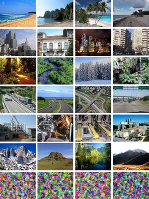  Figure 2

Data Analysis

[I obtained data that had already been preprocessed using AFNI to provide motion correction and to subtract out the temporal mean of each voxel]

First, a spherical searchlight of 81 voxels was centered at every voxel in the brain. Searchlights that did not contain 81 valid voxels (due to being near the edge of the brain, for example) were discarded. An SVM was then trained for each searchlight using the MATLAB implementation of LIBSVM [7]. Each of the 12 runs was held out for cross-validation, one at a time; the accuracy of the SVM was calculated as the average accuracy over these 12 cases. This step was very computationally intensive, requiring approximately 48 hours on a 2.7GHz machine (per subject). Searchlight ROIs were then ranked by accuracy.

A simple form of nonmaximum suppression was used. Any searchlight that overlapped a searchlight with higher accuracy was discarded. The top five ROIs that remained were then selected. In order to interpret these ROIs, it was necessary to match them to anatomical images. Although no anatomical scans were done on the subjects in this study, the distortion matrix mapping the volumes to the MNI template has been calculated. In order to view the selected ROIs, the MATLAB searchlights were exported into AFNI format. FSL was then used to warp the ROIs according to a linear distortion matrix. The ROIs were overlayed on top of the MNI anatomical images using AFNI.

The SVM probability estimates for each ROI were output to text files, and used as inputs for the connectivity analysis. I used a simplified form of the cross-validation method from the original connectivity paper. Each SVM was trained on 11 out of the 12 runs, and then its probability estimates on the held-out run were input to the connectivity analysis to train the weights of the graphical model. The model was then evaluated by re-training the SVM on a different set of 11 runs, and then using its probability estimates on the held-out run as input.

Results

Searchlight Results

Three subjects were analyzed for this project, and the accuracies for their top five ROIs are shown in Table 1.

ROI Number	Subject B7	Subject C4	Subject W5
1	35.9375	32.6389	28.8194
2	32.2917	29.3403	27.9514
3	31.9444	28.8194	27.2569
4	30.7292	28.6458	27.0833
5	30.5556	28.2986	26.9097

These values are all well above the chance level of 1/6 = 16.7%. We can observe that the accuracy has a relatively strong dependence on the specific subject; this could be due to different noise parameters during different scans, or higher-level attentional differences.

The physical locations of the selected ROIs are shown in Figures 3-5. The ROIs for each subject are presented in increasing Z slice location, with numbers indicating their relative SVM accuracy (1 = most accurate). We can identify a number of visual-processing areas among these ROIs. For example, we have identified PPA (B7#2, C4#1 and W5#5), RSC (W5#1), V1(B7#1) and Cuneus (B7#5 and C4#3).

• Searchlight Results
• 

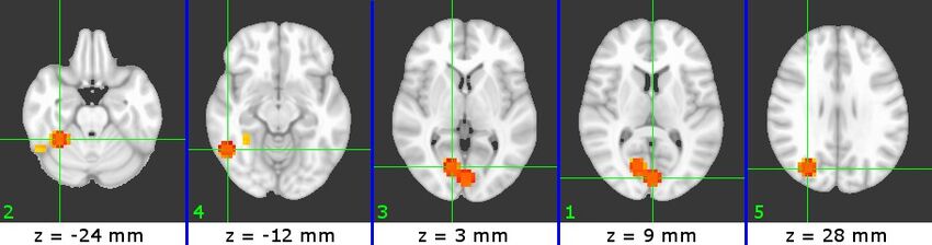  Figure 3 (B7)

• 

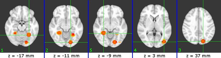  Figure 4 (C4)

• 

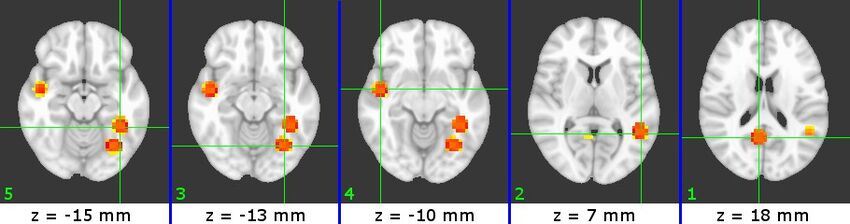  Figure 5 (W5)

Connectivity Results

Since estimating the connectivity requires learning the parameters of a graphical model with hidden variables, it is not possible to find the model that globally maximizes the data likelihood; we must use an iterative algorithm to find a local maximum, which means that the result can be highly dependent on the initial parameter settings. Therefore, I choose 15 different initializations for each subject to find which connections would be learned in each case:

Initial edge value	Subject B7	Subject C4	Subject W5
1		2<->3, 2<->4, 2<->5, 4<->5	1<->2, 1<->4, 1<->5
1.5		1<->2, 2<->3, 2<->4, 2<->5, 4<->5	1<->2, 1<->3, 1<->4, 1<->5
2		1<->2, 2<->3, 2<->4, 2<->5	1<->2, 1<->3, 1<->4, 1<->5, 3<->5, 4<->5
2.5		1<->2, 2<->4	1<->2, 1<->3, 1<->4, 1<->5, 2<->5, 3<->5, 4<->5
3	3<->5		1<->3, 1<->4, 1<->5, 2<->5, 2<->6, 3<->5
3.5	2<->3, 2<->4, 2<->5, 4<->5	4<->5	1<->2, 1<->5, 2<->3, 2<->4, 2<->5, 3<->4, 3<->5
4			1<->2, 1<->3, 1<->4, 1<->5, 2<->3, 2<->4, 2<->5, 3<->4
4.5		2<->3, 2<->4, 2<->5
5		2<->3, 2<->4, 2<->5
5.5	2<->3, 2<->5	2<->3, 2<->4, 2<->5
6	2<->3, 2<->5	2<->3, 2<->5
6.5	2<->3, 2<->5
7		1<->5, 2<->5
7.5	1<->5, 2<->5	1<->2, 2<->3, 2<->4, 3<->4
8		1<->2, 1<->4, 2<->3, 2<->4, 2<->5, 3<->4

We can collect these terms into connectivity matrices by counting the number of times each connection was learned.

B7:

	1	2	3	4	5
1	-	0	0	0	1
2	0	-	4	1	5
3	0	4	-	0	1
4	0	1	0	-	2
5	1	5	1	2	-

C4:

	1	2	3	4	5
1	-	5	0	1	1
2	5	-	9	9	9
3	0	9	-	2	0
4	1	9	2	-	3
5	1	9	0	3	-

W5:

	1	2	3	4	5
1	-	6	5	6	7
2	6	-	1	2	4
3	5	1	-	2	4
4	6	2	2	-	2
5	7	4	4	0	-

One interesting result is that ROI #1 for subject W5 is by far the most strongly connected to other ROIs. Since we identified this ROI as part of RSC, this matches findings in [8] and [5] that RSC plays an important role in scene processing. We also see that PPA in subject B7 (ROI #2) has the strongest complementary connections to other visual areas.

Conclusions

Using a searchlight based on SVM accuracy successfully located brain areas known to be involved in scene processing. Some of the ROIs selected, however, could not be easily mapped to visual areas. These areas can be studied further to identify the role that they play in scene processing.

Using an SVM searchlight is a general MVPA approach that could be applied in many experiments to identify brain areas that are informative about the stimulus. Training using SVMs is simple, since robust libraries exist that can apply complex optimization algorithms to the data. One disadvantage of this method is its computational complexity. For this study, we performed 12-fold cross-validation at every voxel, requiring us to train a total of 12*(~20,000) = 240,000 SVM classifiers for every subject. Although training a single SVM is relatively efficient (~1 second on my 2.7GHz desktop), training this many classifiers requires a large amount of computation. For a larger study, a computing cluster would be required. Note that each classifier is trained independently, so this process can very easily be parallelized over multiple machines.

The connectivity results are difficult to interpret, since the learned connections depend heavily on the initial settings of the parameters. Although I achieved reasonably consistent results, a better approach would involve a much more extensive search of the initial parameter space (e.g. using different initial weight values for different edges). Again, this would take prohibitively long on a single computer, but could easily by parallelized over many computers.

References

[1] Nikolaus Kriegeskorte, Rainer Goebel, and Peter Bandettini. Information-based functional brain mapping. Proceedings of the National Academy of Sciences of the United States of America, 103(10):3863–3868, March 2006.

[2] M. C. Potter. Short-term conceptual memory for pictures. J Exp Psychol - Hum L, 2(5):509–522, 1976.

[3] L. Fei-Fei, A. Iyer, C. Koch, and P. Perona. What do we perceive in a glance of a real-world scene? J Vision, 7(1):1–29, 2007.

[4] R.-E. Fan, P.-H. Chen, and C.-J. Lin. Working set selection using second order information for training SVM. Journal of Machine Learning Research 6, 1889-1918, 2005.

[5] Bangpeng Yao, Dirk B. Walther, Diane M. Beck and Li Fei-Fei. "Hierarchical Mixture of Classification Experts Uncovers Interactions Between Brain Regions." Neural Information Processing Systems Conference (NIPS 2009). December 7-10, 2009. Vancouver, B.C., Canada.

[6] D.Walther, E. Caddigan, L. Fei-Fei*, D. Beck*. Natural scene categories revealed in distributed patterns of activity in the human brain. The Journal of Neuroscience, 29(34):10573-10581, 2009 (*indicates equal contribution)

[7] Chih-Chung Chang and Chih-Jen Lin, LIBSVM : a library for support vector machines, 2001. Software available at http://www.csie.ntu.edu.tw/~cjlin/libsvm

[8] B. Chai†, D. B.Walther†, D. M. Beck∗, and L. Fei-Fei∗. Exploring functional connectivities of the human brain using multivariate information analysis. In NIPS, 2009. (†, ∗ indicates equal contribution).

Software used: MATLAB, Visual Studio 2008, AFNI, FSL