David Gal
Introduction
This project aims to realize a fast implementation of the novel L3 image-processing pipeline developed by Steven Lansel at Stanford University.
Background and Motivation
Moore’s law has resulted in unprecedented scaling of both the technology and economy of the semi-conductor industry. Among other advancements, semi-conductor scaling has enabled CMOS imaging sensors to reach resolutions of 10s of millions of pixels (megapixels). Traditional research in imaging technology has often focused on improving key metrics of these sensors such as SNR, power consumption, and cost. The abundance of pixels in today’s commercially available imaging sensors has become something of a marketing campaign and competition for leading camera manufacturers. At present both Canon and Nikon offer consumer cameras with more than 20 megapixels. Given a monitor with 72 dots per inch (DPI) such cameras are capable of producing images that at full size occupy in excess of 60” in a single dimension. As a result of what has become “overkill” for the typical consumer researchers have begun to consider other uses of pixels in imaging sensors. One such utilization of the pixels on a sensor is the realization of novel color filter arrays (CFA).
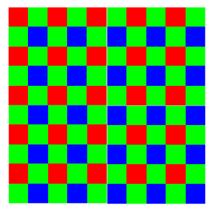
The ubiquitous Bayer pattern seen in the figure below has served both the consumer and professional photographic community well. Its design and consideration for the human visual system – namely high spatial sampling of green wavelengths – has rendered it a universally accepted standard in still camera design. Numerous papers have been published on the Bayer pattern’s merits as well as algorithms for demosaicing, denoising, and color transforming its resultant sensor data.
The Bayer pattern is, however, not without its limitations and despite its wide adoption should by no means be considered the end all and be all of CFA design. Researchers have considered countless designs of CFA patterns in the past. Coupled with the advent of such pixel rich sensors new CFA patterns may well find their way into the consumer market soon. One such considered improvement to CFA design is the addition of a “white” pixel in the array. Such a pixel would filter at near infrared frequencies and provide a true luminance channel. With this additional channel low-light photography could occur with faster shutter speeds thus reducing blur. Additionally it’s possible that higher dynamic range images could easily be captured.
The trouble with novel CFA design is not, however, in the design of the array itself. It is in fact in the design – or rather lack of design – of the image-processing pipeline that transforms sensor data to an image on a screen. As aforementioned countless methods for demosaicing, denoising, and color transformation exist for the Bayer pattern, but for a novel CFA pattern there is no reason to assume such algorithms exist. The necessity of such algorithms can be a major bottleneck in novel CFA research. Without the requisite transformation pipeline there is no way to properly evaluate novel CFA design.
L3 Motivation and Background
The L3 pipeline developed by Steven Lansel aims to mitigate this bottleneck. The L3 pipeline is capable of performing demosaicing, denoising, and color transformation with the application of a single filter thus ameliorating the need for a novel pipeline for every novel CFA pattern.
L3 stands for local, linear, and learning. Indeed the L3 algorithm is all of these. There are two fundamental components to the L3 algorithm – a regression stage that builds libraries of filters and an application stage that utilizes these filters to perform image processing.
The regression stage involves taking several images with any CFA pattern at different illuminant levels. L3 categorizes 9 x 9 sections of an image known as patches into two fundamental types – flat patches and texture patches for smooth and edged surfaces respectively. Knowing what the ideal image should look like a novel regression algorithm creates an ideal filter set for various structural elements within an image. While the filter tap coefficients indeed change for novel CFA designs, the mechanics of applying the filters do not. The burden of creating the optimal filter set is left to the regression algorithm, but is largely agnostic to the CFA design.
For every color element in the CFA pattern a filter library is created. In the case of a Bayer pattern there are four filter libraries – one for red, two for green, and one for blue. Figure 2 shows the contents of a filter library.
As seen there are several different filters in a single library. All filters are applied using the standard correlation method (convolution without kernel flipping) as seen in Equation 1:
- Equation 1
As illustrated by equation 1 for each filter application there are a total of 81 multiply accumulate operations. In this project all data is assumed to be IEEE 754 floating point.
The final filters – the flat and texture filters – must be applied to a patch that is rotated and transformed to be in a canonical layout with the darkest area of the patch in the upper left corner. Patches may be flipped horizontally, vertically, translated across the major diagonal, or some combination of these transformations.
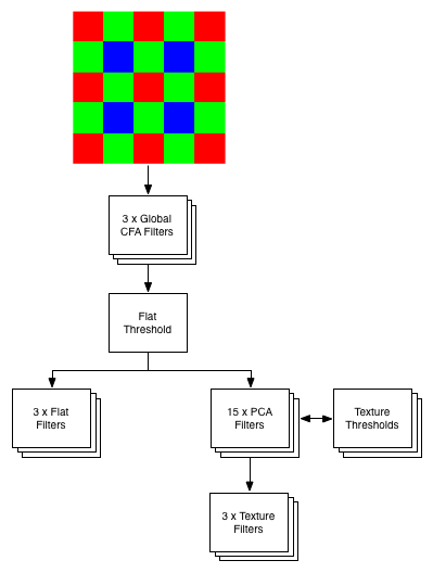
The three Weiner filters known as Global CFA filters are utilized to give a rough estimate of the patch type – either texture or flat. A patch is determined to be flat if the result of the average of the difference between a patch and its global CFA results is greater than a threshold. If a patch is determined flat then the three flat filters give estimates for X, Y, and Z. If a patch is determined to be textured then N PCA filters are utilized to determine the texture type. In the case of this project there are 16 texture types which means that there are 15 PCA filters. The PCA filters are organized in a binary tree fashion such that only 4 PCA filters need to be applied to determine the ultimate texture type (one for each level in the PCA tree). For each application of a PCA filter there is a corresponding threshold which indicates which next node PCA filter should be applied. In this way the binary tree of PCA filters is walked until the final texture type is known. Finally the appropriate texture filters can be applied to give estimates in X, Y, Z color space. In its current iteration the L3 pipeline is implemented entirely in Matlab.
Algorithm Analysis
Figure 3 graphically depicts the per patch algorithm utilized to give X, Y, Z color estimates at a given pixel.
The requisite computations for a flat patch are:
- 3 x 9 x 9 floating point MAC - for Global CFA Filters
- 3 x 9 x 9 floating point MAC - for Flat Filters
The requisite computations for a texture patch are:
- 3 x 9 x 9 floating point MAC - for Global CFA filters
- 4 x 9 x 9 floating point MAC - for PCA filters
- 3 x 9 x 9 floating point MAC - for Texture FIlters
As seen this algorithm is quite computationally intensive. For a 500 x 500 image there are at least 162 million floating point multiply accumulate operations. For a 3-megapixel image there are 2 billion floating point multiply accumulate operations. Clearly there are a proportional number of memory references as well. It should be noted that the algorithm actually scales relatively well. Adding, for example, more levels to the PCA tree does not significantly contribute to computational complexity. The largest contributor to computational complexity is, in fact, the size of the filter/patch pair.
As Matlab is an interpreted environment such computational complexity can result in very slow algorithmic execution. A faster implementation would be useful for researchers interested in novel CFA patterns.
Towards a Faster Implementation
Figure 3 also indicates a huge amount of potential thread and data level parallelism, which Matlab is likely not exploiting. Such parallelism fits well within the modality of super-scalar processor architectures, but even more so with modern graphics processors (GPUs), which can be thought of multi-cored, threaded vector architectures. As a baseline reference a pure CPU implementation was realized utilizing C++ and the OpenCV libraries. As the L3 pipeline involves a large amount of matrix-based operations the OpenCV libraries, which are based on the BLAS libraries, were utilized in the implementation. OpenCV libraries are open source and are accompanied by relatively good documentation.
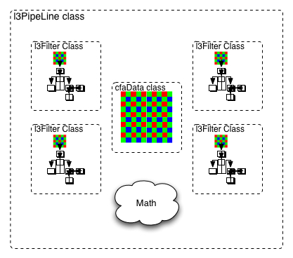
A three-class model was chosen for the implementation. As seen in Figure 4 a cfaData class, l3Filter class, and l3PipeLine class were realized.
The cfaData class contains:
- A matrix of sensor data
- A texture map matrix
- A flip map matrix
- Functions to load sensor data and parameter from Matlab generated text files
The l3Filter class contains:
- 3 x Global CFA filters
- 1 x Flat threshold
- 3 x Flat Filters
- 15 x PCA filters
- 15 x Texture thresholds
- 16 x 3 Texture Filters
- Methods to load filter data and parameters from Matlab generated text files
The l3PipeLine class contains:
- 1 x cfaData
- 4 x l3Filter
- Methods to process the pipeline and output Matlab read text files with results
Results
The C++/OpenCV implementation of L3 is a promising first step in realizing a truly data and thread parallel implementation on a GPU. As compared to the Matlab implementation the C++/OpenCV implementation realized roughly a 6x speed up on average. All images processed in this project were 401 x 481 pixels in size. On a macbook pro with a 2.5 GHz Core 2 Duo with 4 GB 667 MHz DDR2 SDRAM the average Matlab execution of a single L3 image was found to be 11.59 seconds compared to an average 2.06 seconds using the C++/OpenCV implementation. Much of the execution time spent for the C++/OpenCV implementation was utilized for memory allocation and temporary storage of a patch for the purposes of flipping and transposing. The serialization of such a memory bottleneck would be greatly reduced with the facilitation of a GPU architecture.
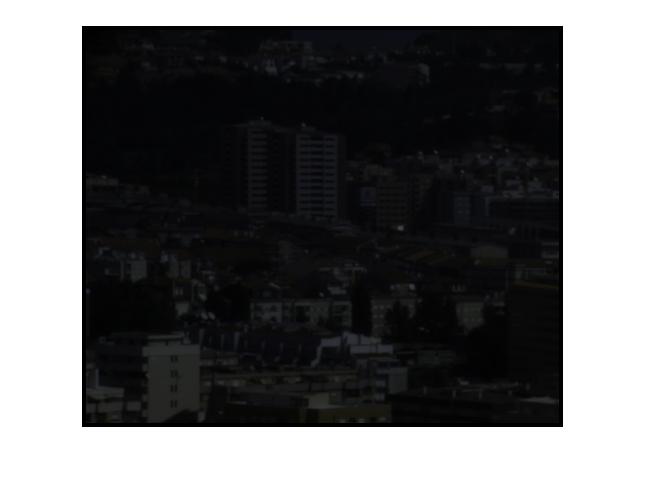
Figure 5 shows an output image from the C++/OpenCV implementation.
Utilization of the C++/OpenCV L3 implementation is trivial from the programmer’s perspective. Simply declare a new instantiation of an l3PipeLine and execute the process method:
l3PipeLine *pipe = new l3PipeLine(“..\..\”);
pipe->process();
Future Work
There is a significant amount of work that can and should be done to build upon this progress. Firstly all the Matlab I/O should be overhauled to use the Mathworks header files for reading and writing .mat files. The current iteration assumes a precise text file format and cannot tolerate any deviations from this format. As the author will attest it is error prone and inefficient.
The existing code base needs more commenting and cleaning. Finally a GPU implementation using either NVIDIA’s CUDA or OpenCL should be realized. A significant amount of the author’s time was invested in an attempt to create a GLSL shader stack implementation. This involved heavy multi-texturing for proper scaling and ultimately it was decided that GLSL best be used for what it was designed.
Credits/Resources
The author would like to thank Steve Lansel for answering numerous late night emails and questions.


