Deblurring sensor images using known psf models

Project Team: Jona Babi, Rakesh Ramesh, Dimitris Papadimitriou

In this project, we aim to deblur the image produced by the sensor using the known PSF model. We extend the study to different types of psf models: shift-invarianat, shift-vairant and wavelength-dependent PSFs, and perform noise-margin analysis for different types of sensor noise: Read noise, Pixel Response Non-Uniformity (PRNU) and Dark Signal Non-Uniformity (DSNU).

We will then use the developed model to frame answers to interesting questions like:

• How well can the image be sharpened using deconvolution if PSF is known?
• Which type of PSF-model provides us sharper deblurred images?
• What noise-margins can a PSF-model tolerate for deblurring?
• What type of noise can be tolerated by the sensor?

Introduction

Image restoration refers to the process of removal or minimization of known degradations in an image. This includes deblurring of images degraded by the limitations of the sensor or its environment, noise filtering, and correction of geometric distortions or non-linearities due to sensors. One of the reasons why the degradation happens is that most lenses including the human eye lens are not perfect optical systems. If an exceedingly small dot of light, is projected through a lens or an image system, the output will include the point surrounded by a small amount of blur. The question is how can this degradation be represented? The answer is using the Point Spread Function (PSF).

The PSF describes the response of an image system to a point input and it is analogous to the impulse response of filters [1]. A point input, represented as a single pixel in the “ideal” image, will be reproduced as something other than a single pixel in the “real” image. The output image may then be regarded as a two-dimensional convolution of the “ideal” image with the PSF: $g=f*PSF$ (superposition principle). The PSF can be represented as a 4D-function, PSF(x, y, $f_{x}$, $f_{y}$, $\lambda$), which depends on the image plane coordinates (x,y), the original field position ($f_{x}$, $f_{y}$) and the wavelength $\lambda$. There are different types of PSF models, one can use to represent the blurring by the optics which are essentially simplifications of the 4D-function by fixing some of the parameters. For this project, we consider 3 PSF-models: Shift-Invariant PSF, Shift-Variant PSF and Wavelength-dependent PSF. Shift-Invariant PSF-model assumes that the PSF is the same over the original scene and thus the final image is just a 2D-convolution of the scene and the PSF. Shift-Variant PSF-model relaxes that constraint which means the PSF is dependent on the position of the pixel in the original image. We represent Shift-Variant PSF using a matrix of Shift-Invariant PSF that is indexed by the field position from the original scene. In Wavelength-dependent PSF model, we vary the PSF for different wavelengths to capture the chromatic aberration due to the different blur functions for different wavelengths.

One approach towards image quality improvement is using the lens point spread function (PSF) to deconvolve the image so that the aberrations can be reduced. This step requires knowledge of the underlying PSFs, the acquiring of which (usually by taking photos of pinhole arrays) is laborious and prohibitive. Alternatively, one can simulate the PSF if the lens model is known. So it is possible to measure and improve the performance of an imaging system by running simulations without any immediate need of hardware usage. Such simulation capabilities allow almost effortless visualization of the image quality impact of component substitution, or modifications to tolerances or component specification. Consequently, the construction of precise image capturing simulations is an active research area due to its significance in image quality improvement. [2] [3]

Methods

Tools

We used the Image Systems Engineering Toolbox (ISET) [4] to perform all our analysis for the project. We utilized the inbuilt Lucy-Richardson deconvolution method [5] to perform the deblurring. Lucy-Richardson method iteratively deconvolves the blurred image $I$ and tries to maximize the likelihood of the deblurred image having been blurred by the supplied PSF to obtain $I$. We also use the zemax example optics (rtZemaxExample.mat), found under ISET data, for the Shift-Variant and Wavelength-dependent study.

Steps

Simulation

We simulated the image system pipeline from the scene to the optical image to the sensor image using ISET. Then we deblur the sensor image and compare it to our original image to asses the quality of our deblurring method. Broadly, we can separate our simulation into the following steps:

• Create a scene (point-array / cameraman / lenna)
• Load the zemax ray trace PSF data (aspherical 2mm lens)
• Generate the zemax optical image
• [ Create optical image with a shift invariant zemax psf ]
• Create a sensor (monochromatic / bayer)
• [ Modify the sensor noise attributes ]
• Capture the sensor image
• Deconvolve the sensor image using the known psf
• Compare the deblurred image with the original image (PSNR, SSIM)

Simulation Flow

Analysis

After setting up the simulation infrastructure and adding in the PSF models to the flow, we perform the following analysis for the purpose of this project:

• Analyse how well the deblurred images compare to our original image with different PSF models (Shift-Invariant, Shift-Variant, Wavelength-dependent)
• Analyse the deblurring quality for different types of scenes - Sparse (Point-array) and Dense (Cameraman, Lenna)
• Analyse the noise margins on the image that can be tolerated by the blur function
• Analyse the noise margins for different types of sensor noise (Read noise, PRNU, DSNU)

Image Quality Metrics

In order to measure the quality of the blurred and deblurred images we will use two of the most widely used metrics, the Peak Signal to Noise Ratio (PSNR) and Structural Similarity Index (SSIM).

• Peak Signal to Noise Ratio (PSNR):

The Peak signal to noise ratio is the most commonly used image quality metric and high values almost always signify a better reconstruction of the original image. It is defined as follows:
$PSNR=20log_{10}{\frac {MAX_{i}}{\sqrt {MSE}}}$

with the mean squared error being
$MSE={\frac {1}{mn}}\sum _{i=0}^{m-1}\sum _{j=0}^{n-1}[I(i,j)-K(i,j)]^{2}$.

where I,K and $MAX_{i}$ are the control image, output image and the maximum image pixel value of the image respectively.

• Structural Similarity Index (SSIM):

The structural similarity index is a measure of similarity between images by taking into account structural information. The definition is:

$SSIM(x,y)={\frac {(2\mu _{x}\mu _{y}+c_{1})(2\sigma _{xy}+c_{2})}{(\mu _{x}^{2}+\mu _{y}^{2}+c_{1})(\sigma _{x}^{2}+\sigma _{y}^{2}+c_{2})}}$

with $\mu _{i},\sigma _{i}$ and $\sigma _{ij}$ being the mean, variance and covariance and $c_{i}$ some constant to avoid division by a small number. The higher the SSIM value the better the reconstruction of the image.

Results

PSF Model: Shift-Invariant; Scene: Point-Array

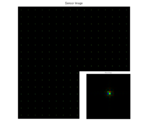
In the first experiment, we create a point-array scene (1 wavelength only) and blur the scene using a shift-invariant PSF. In order to blur this image uniformly we used only one of the PSFs that we obtained from the optics object of the Zemax file (which returns 37 by 12 distinct PSFs). The blurred optical image and the sensor image can be seen here:

• 

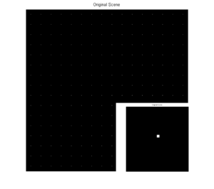  Original Scene

• 

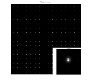  Optical Image (PSNR=25.76, SSIM=0.87)

• 

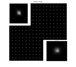
  Sensor Image (PSNR=27.40, SSIM=0.86)

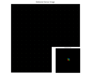
We note that all the pixels of the image are blurred in exactly the same way because the PSF is shift-ivariant. In order to deblur the sensor image we deconvolve it by using the same PSF that we used to blur the original scene. The deblurred image can be seen here:

• 

  Sensor Image

• 

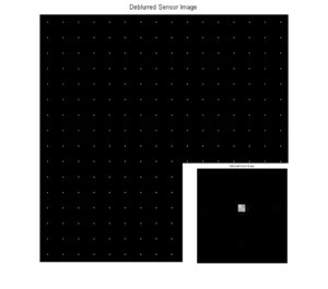  Deblurred Sensor Image (PSNR=28.22, SSIM=0.94)

We observe that the deblurring results in an sharper image with higher PSNR value. However this image slightly differs from the original one because the shift-invariant optics in ISET is implemented as an Optical Transfer Function (OTF) which performs the convolution in the fourier domain, i.e. OTF is multiplied by the FFT of the original image and then IFFT to obtain the blurred image. When the inverse fourier transform is applied, ISET keeps only the magnitude of the resultant blurred image and loses the phase of the complex value. Hence, the final image is the deconvolution of the magnitude of the IFFT which doesnt reproduce the exact original image but is very close to it.

PSF Model: Shift-Variant; Scene: Point-Array

In the shift-variant case, we use the field position dependent PSF to blur and deblur the image. The effect of using such PSFs can be seen in the resulting images in which the blur is clearly nonuniform among the pixels. The resulting deblurred image is significantly improved in quality both visually and with the PSNR and SSIM metrics.

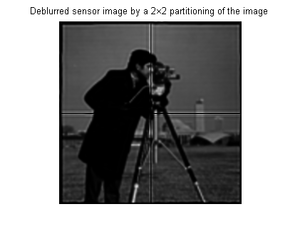
The algorithm we use to perform the deblurring with a shift-variant PSF is partitioning and deconvolving by parts. To put it more precise, we first separate the sensor image into a number of sub-images ($k_{1}\times k_{2}$). Then we deblur each part of the image by using the PSF that corresponds to each field position and finally we merge the images in order to acquire the complete image. In the case that we present we used a $16\times 4$ partitioning. Given the simple structure of the image there is no need to perform any sort of smoothing on the output image since the boundary artifacts do not affect the quality of the image. The sensor and the deblurred images are shown below:

• 

  Sensor Image (PSNR= 22.38, SSIM=0.54)

• 

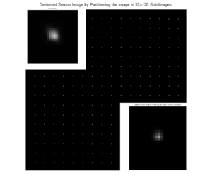  Deblurred Sensor Image (PSNR=26.98, SSIM=0.85)

PSF Model: Shift-Invariant; Scene: Cameraman

We extend our deblurring experiments further by testing them on more denser scenes. In this experiment we use the monochromatic cameraman image and deblur with a shift-invariant PSF. The original image, along with the blurred Zemax figure are shown below:

• 

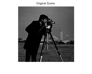  Original Scene

• 

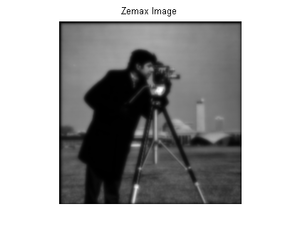  Zemax Blurred Optical Image

In order to deblur the sensor image that we obtain we use the same field position independent PSF that we used to blur the image. The deblured image is significantly improved compared to the sensor image, but it is clearly is not as sharp as the original one since it has lower contrast. Both the sensor and the deblurred image are as shown below:

• 

  Sensor Image (PSNR=22.45, SSIM=0.67)

• 

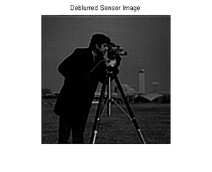  Deblurred Sensor Image (PSNR=26.92, SSIM=0.86)

PSF Model: Shift-Variant; Scene: Cameraman

The blurring in this case is not shift-invariant as we use a field position dependent PSF to blur the image. The deblurring is carried out as described in the point array example and the deblurred image that we obtain along with the sensor image can be seen here:

• 

  Sensor Image (PSNR=)

• 

  Deblurred Image (PSNR=18.53, SSIM=0.62)

However, we observe that our partitioning method also adds noise in the form of edge artifacts that were not present in the blurred image. These artifacts show up because the deconvolution cannot produce proper results for pixels that are close to the boundary of the image. For this reason we need to perform smoothing in the deblurred image in order to avoid such discontinuities. We tried a number of methods for this cause.

First we used edge detection algorithms to detect the sharp edges of the image and delete them. However, this approach resulted in losing information about the already existing edges in the image. Furthermore, uniform gaussian smoothing on the entire image or in the noisy edges of the image did not lead to solid results. The method that gives the best results, according to both visual and PSNR criteria is the one in which we augment each sub-image by replicating the row and column of pixels that are in contact with another sub-image a few times. Then we perform deconvolution on each of these augmented sub-images and merge them together by ignoring the replicated pixels so that we eventually get an image of exactly the same dimension as the initial one. One instance of $2\times 2$ partitioning of the image can be seen here:

• 

  Deblurred Image (PSNR=18.53, SSIM=0.62)

• 

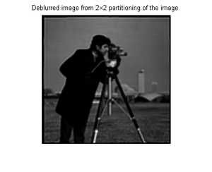  Smoothed Deblurred Image (PSNR=20.04, SSIM=0.67)

Looking closely we can still detect the edge artifacts which are now very limited. For this specific image that we are using dividing it into parts smaller than $4\times 4$ does not result in significant improvement in the PSNR or SSIM metric. We also observe that the deblurred image without smoothing has lower PSNR and SSIM values than the blurred one, something that signifies the effect of the edge artifacts.

PSF Model: Wavelength-dependent; Scene: Point-Array

In this experiment, we use a wavelength-dependent (shift-invariant) PSF to blur the original scene and use a bayer filter to capture the blurred sensor image. The original sensor image and the deblurred image are shown below:

• 

  Sensor Image (PSNR=31.43, SSIM=0.93)

• 

  Deblurred Image (PSNR=31.01, SSIM=0.94)

We notice that the bayer sensor produces bayer pattern for the single point pixel along with the blurring for each wavelength which can be noticed in the color rings surrounding the bayer pattern. The deblurred image produces a better image than the sensor image but the interpolation due to the bayer pattern leads to lower PSNR and SSIM values when compared to the original scene.

PSF Model: Wavelength-dependent; Scene: Lenna

We extend the wavelength-dependent study for a larger and denser chromatic image of Lenna. The scene used in our experiments consists of only 3 wavelengths (R-650, G-550, B-450) of the original image to speed-up the blurring and deblurring process. The original scene, the sensor and the deblurred images are as shown below:

• 

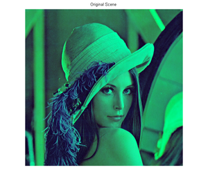  Original Scene

• 

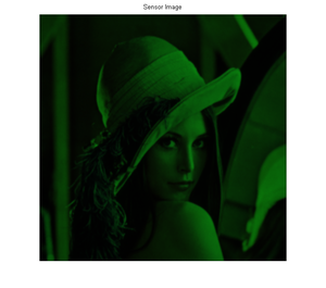  Sensor Image (PSNR=11.38, SSIM=0.068)

• 

  Deblurred Image (PSNR=11.23, SSIM=0.062)

We notice that the sensor image is significantly blurred first by the optics and then by the bayer filter. The bayer filter destroys the structural similarity to the original scene as seen with our SSIM and PSNR metrics. The deblurred image isn't any different from the sensor image and the effects of the bayer filter could not be undone to produce better deblurring.

Noise Margins

The deconvolution algorithm used to deblur the sensor image is sensitive to noise. Non-ideal sensor adds noise to the sensor image. The different types of noise that affects the sensor are given below:

• Shot Noise
• Read Noise
• Pixel Response Non-Uniformity (PRNU)
• Dark Signal Non-Uniformity (DSNU)

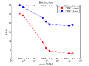
Noise Margin analysis characterizes the sensitivity of the deblurring scheme to the various types of noise. We extend the simulation infrastructure for our previous experiments and vary the magnitudes for the Read, PRNU and DSNU noise and observe the quality of our sensor and deblurred image. We do not vary the shot noise since that is a characteristic that is dependent on the number of photons that are present and is modeled in our noise margin analysis by default. The plots for the PSNR of sensor and the deblurred image vs the noise levels and different types is shown below:

• 

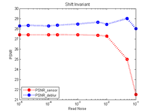  Read Noise

• 

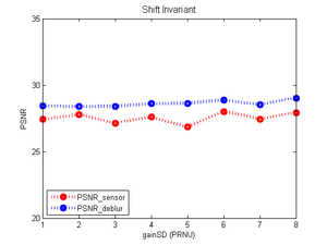  PRNU

• 

  DSNU

There are a number of interesting observations we derive from our plots. We observe that the PSNR metric responds in the same way for both the sensor and deblurred images, i.e. there is a strong correlation between the two as expected. Secondly, we see that the sensor image degrades much faster with the read noise while our deblurred is able to withstand the read noise to a certain degree until the image completely degrades (100x). However, we see no noticeable pattern for the PSNR of the sensor and the deblurred image when we varied the PRNU level which implies that the non-uniformity is not a big factor when we consider deblurring. Finally, the DSNU noise in the sensor is the biggest quality determining factor. The quality of the sensor and deblurred image decreases sharply with increase in DSNU noise. Note that similar trends can be observed for the SSIM metric and the shift-variant PSF case.

Conclusions

The scope of the project was to provide answers on how well we can sharpen an image if we know the underlying PSF under different PSF models and the different noise parameters. Given a field position independent PSF and no additional sensor noise we observed that we could achieve a significant improvement in the sharpness of the image. In the case of shift-variant PSFs we had to partition the image and deblur by using a different PSF for each part. A small partitioning has a significant impact on the PSNR but partitioning the image into very small images does not give considerable further improvement, mainly because the edge artifacts start to have greater effect on the quality. In the wavelength dependent PSF study we didn't manage to get a deblurred image that was improved compared to the sensor image, something that is attributed to the effects of the bayer filter. The noise margin analysis also provides us the 3 interesting inferences: the sensor image can tolerate read noise to an extent for deblurring, the sensor image and deblurring is not affected by the PRNU level and finally the sensor image and deblurring is heavily dependent on the DSNU level which plays a big factor in quality of the image.

To conclude, image restoration is a rapidly growing field that has helped correct the physical limitations in the modern lens technology, one of which is blurring. In this project, we have unconvered some of the aspects to deblurring the image produced by the sensor and under different PSF models and noise margins and we believe that there is still a lot to explore in this area to get very precise accurate images that are closer to the original scenes for a better image system for the future.

References

• Wikipedia : Point Spread Function
• Wikipedia : Peak Signal to Noise Ratio (PSNR)
• Wikipedia : Structural Similarity Index (SSIM)
• Mathworks : Lucy-Richardson Algorithm (deconvlucy)
• Image Enhancement using Calibrated Lens Simulations (Y.Shih,B.Guenter and N.Joshi)
• Image Capture Simulation Using an Accurate and Realistic Lens Model (R.Short,D.Williams and A.Jones)
• Joyce Farrell, Peter B. Catrysse, Brian Wandell, “Digital Camera Simulation”, http://white.stanford.edu/~brian/papers/pdc/2012-DCS-OSA-Farrell.pdf

Appendix I

• Source Code : File:Psych221 Deblurring Source Code.zip
• Project Presentation : File:Psych221 deblurring presentation.pdf

We also had to modify some of the already written ISET scripts. More specifically, the lines 119-121 of the \opticalimage\optics\shiftinvariant\siSynthetic.m have to be commended.

Appendix II

Our group met frequently to discuss and understand ISET (mainly Rakesh Ramesh) before setting up the simulation infrastructure for the experiments. Then we carried out the experiments in parallel and analysed each part individually and as a group to draw concrete conclusions. We divided the project workload very broadly as listed below:

Rakesh Ramesh: Shift-invariant PSF study, Wavelength-dependent PSF study

Jona Babi: PSF-size influence study, Noise margins analysis

Dimitris Papadimitriou: Shift-variant PSF study, Edge Artifact smoothing, Image Quality Metrics

We worked on the group presentation and the wiki together as a group.

Acknowledgements

We would also like to thank Joyce Farrell and Andy Lin for their helpful guidance in the duration of our project.