Design and Evaluation of Demosaicing Algorithms for RGBW CFA

Introduction

Nathan Staffa

Engineering in the commercial imaging sector knows nothing of patience; if anything, the pace at which camera technology is growing is faster than ever. Improvements are being made at an incredible pace across the entire range of the imaging system. One aspect that has not seen this pace, however, is that of the color filter array (CFA).

Color filter arrays are small arrays that sit in a camera immediately above the sensor. CFAs filter incoming light, absorbing a range of wavelengths and allowing a desired range through to the sensor, effectively choosing only certain colors. The pattern in a CFA is typically designed in such a way that each sensor pixel receives light filtered through only one filter, with the total number of individual filters equaling the number of sensor pixels. Thus, the pixels can be considered color-coded. This is a key step in the entire image processing pipeline.

As mentioned, CFAs have not seen much development, and in fact the go-to standard utilized by nearly all consumer level cameras has seen itself roughly constant since its introduction forty years ago: the Bayer color filter array. Introduced in 1976 by Bryce Bayer, this simple repeating 2x2 arrangement of red, green, green, blue, has been a remarkably stable feature. Though there has in the past been a moderate level of interest in other designs, there was not much perceived reason to stray from the Bayer standard. Recently, however, there has been an increased interest in the design of new and novel color filter arrays, with the promise of increases in several aspects of imaging, from multispectral capture to increased resolution to increased dynamic range.

High dynamic range

One of the major hurdles that faces imaging is the problem of dynamic range (DR), the difference between the brightest and darkest parts of a scene. Though a camera can capture a reasonably wide DR, that data must be stored, resulting in a first loss of DR, and then ultimately displayed, resulting in the largest loss of DR. The issue of being unable to display HDR images without DR compression and tonemapping is one under current research. This project does not address the problems of HDR rendering on LDR displays, but rather considers the ability of the camera sensor to capture high quality signals in regions of low-light.

Average pixel values per channel for Crothers Image

Average pixel values per channel for dark region in Crothers Image

Normally, as light passes through the CFAs, photons are absorbed by the filter, resulting in a smaller number photons on the sensor, leading to a lower signal. This lower signal often falls beneath the noise floor of the sensor, in which case no usable or reliable information can be recovered from these pixels. If however a subset of pixels are transparent (referred to as clear or white), with a high, broadband spectral sensitivity, these previously problematic areas now become more manageable: with greater number of photons, SNR is increased, and the signal may rise above the noise floor, allowing for the obtainment of signal where previously there was none. This is one of the primary reasons for manufacturer experimentation with RGBW (red, green, blue, white, or RGBC, clear) CFA configurations.

But with new CFA designs, the more-or-less solved problem of demosaicking increases in complexity.

Demosaicking RGBC

When a sensor reads out an image, it reads pure signals, mindless toward any filter arrangement. A raw image therefore has no colors; it is only a set of pixels ranging from dark to light. To extract a colorful reproduction of the captured scene, the image processing pipeline must apply knowledge of the configuration of the color filters which match up with those read values. Each pixel, however, is a measure of only one color channel. Therefore the color-coded image at this stage is a repeating pattern of pure red, green, blue, or grey pixels, as determined by the CFA. This is what is referred to as a mosaic. Demosaicking is the process of inferring from each of these mosaicked color channels the values of all the other channels at all points.

Numerous approaches to demosaicking exist, including spatial domain methods acting on a per-channel basis (linear interpolation being among the most simple), spatial methods on a cross-channel basis, and frequency domain methods, relying on demultiplexing overlapping spectra. They all present numerous advantages and disadvantages, but in each case, the problem for the RGBC CFA is the same: how do you use the white pixel data?

Answers to this question have not been decided by the field it seems, and results of applied usage of novel CFAs with a clear pixel have been met with mixed reaction. This serves to highlight the crux of the problem: utilizing the clear pixel effectively is hard.

Summary

We test a prototype novel CFA design from manufacturer OmniVision utilizing the RGBC (C for clear, not cyan) modality described above. Current literature has not explored at length the demosaicking problem for RGBC, and as such, exploration into possible demosaicking methods is explored. Particular attention is paid to demonstration of proposed potential advantages granted from the presence of the clear pixel, most notably the increase in contrast at low-levels.

It is worth noting that though a full range of bracketed exposures were captured for all scenes, no processing was attempted on more than a single exposure at a time. Exposure bracketing is not especially relevant to the RGBC device: where the RGBC camera offers advantages is in the range it can capture within a single shot. If you are going to take a bracketed set and combine, then there is little to be gained from RGBC, thus an RGB camera would be sufficient. The only possible advantage it would allow for is allowing slightly more on the low-end of the lowest-exposed shot of the group; the rest would have been covered by the well-exposed RGB pixels.

Image capture

Working with a prototype proprietary imaging sensor imposes certain restrictions on usability. Concretely, all management of imaging parameters must be manually controlled from an external computer via a USB link. The company, OmniVision, provided a software package, OVTAPanther, to mediate this process.

Sensor parameters

Through OVTAPanther, control was granted in the following areas: image resolution, exposure time, and sensor gain. (Also granted control of were several other parameters not relevant to the work at hand.) As the lens was a small generic lens fixed in place above the sensor, no control was possible over focal length or aperture.

It was important to use the maximum resolution of the sensor, and to be consistent through captures, as at this point neither the tessellation of the CFA was known, nor was it known if the edges of smaller resolutions would exactly between CFA repetitions. If the latter case turned out to be false, the overall alignment of the CFA pattern throughout the image would be shifted, throwing off most demosaicing algorithms which rely on set, known mosaics.

Though sensor gain and exposure time would both allow control over overall exposure, the behavior of the gain of this sensor and its effects on the image were not well characterized, therefore a choice was made to use the lowest gain possible (1x in OVTAPanther, ostensibly no extra digital gain) in order to eliminate this variable from affecting results. With both aperture and gain removed, our control over exposure then rested solely on exposure time, or shutter speed, which would be the primary variable of interest during capture.

Capture setup and scene selection

An example of image setup

In order to stabilize the small sensor over the course of capturing multiple exposures, the device was secured using a small vise-like mount which was then attached to a tripod mount plate for positioning. The device was then connected via USB to a small laptop. Proper orientation of the device was determined through the live preview display of OVTAPanther.

Due to the novel nature of the device, pure simulation of the mosaic using standard test images was determined to inadequate. Particularly due to the potential of the RGBW in regards to dealing with high dynamic range scenes, it was important not to use test images from non-HDR capable devices, but rather capture true HDR scenes in reality. From these scenes, the HDR potential can be tested.

In pursuit of the goal of HDR capture, HDR scenes were selected around Stanford campus. In order to satisfy the criterion, scenes were required to have characteristics that would challenge most standard imaging devices. Therefore priority was given to scenes that paired very bright regions (often due to strong sunlight) with comparatively dim regions (often in sun shadow, or building interiors). Several scenes were selected:

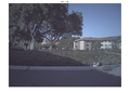
• The Crothers courtyard -- Direct sun on field and buildings, paired with dark shadows from building and trees.
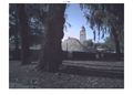
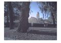
• Hoover Tower -- Brightly lit tower and construction area, with strong shadows from large tree.
• Main Quad arcade -- Highlights from direct sunlight with darker regions in the ceiling of the arcade
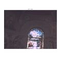
• Memorial Church ceiling -- Strong diffuse lighting from skylight, paired with dark from the other ceilings in the church
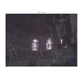
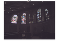
• Memorial Church stage -- Bright regions in the stained glass, with dark regions in the ceiling and the shadows of the statue.
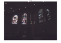
• Memorial Church side -- Brights in the stained glass, shadows in the pews and chairs.
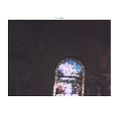
• Memorial Church doorway -- Highlights in the sky and outdoor quad, with near-black regions in the interior of the church.
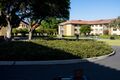
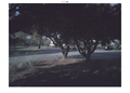
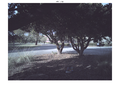
• Roundabout Trees -- Highlights from the path and building, with most of the image in shadow from the trees

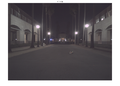
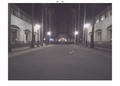
Several images were also taken at night. While night images often are also HDR, these images also allow comparisons to standard imaging devices in terms of requisite exposure: Would the white pixels of the image allow for shorter shutter speeds while still recovering reasonable signal? Several night images were selected:

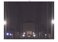
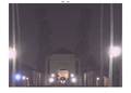
• Main Quad arch -- Good light on the arch, with dimly lit Hoover Tower and roofs of arcades
• Main Quad lamp -- Strong direct light from the lamp, with nearly everything else underexposed.
• Path from Engineering Quad -- A good mix of moderately lit regions with dark throughout

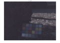
Present in each image is the Macbeth ColorChecker used for reference and color-correction. The ColorChecker was typically placed in darker regions of the scene, as these would be the regions most challenging for accurate color rendition.

Images were taken bracketed over a range of exposure lengths in order to maximize coverage and potential. Though true intensity of light was not measured at the time of capture, it can be estimated through knowledge of the spectral response curves and the range of exposures captured.

It is particularly important to note that the capture of these scenes through this sensor allow for work on many novel image processing techniques for this CFA architecture. Our work is only a small attempt at using the new data available in such a design, and I hope that others will build off this dataset and design even better algorithms for dealing with such data.

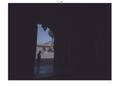
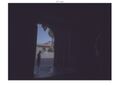
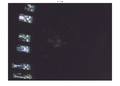
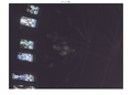
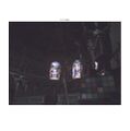
The reference images below are simply meant to give an idea of the appearance of the scenes and the HDR challenges each present. These images were not taken bracketed or in any HDR mode, and are purely for visual understanding.

• Scene reference images, taken with consumer camera
• 

  Crothers Courtyard

• 

  Hoover Tower

• 

  Main Quad arcade

• 

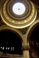  Memorial Church ceiling

• 

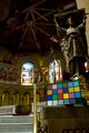  Memorial Church stage

• 

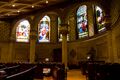  Memorial Church side

• 

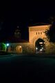  Main Quad arch

• 

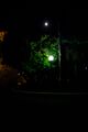  Main Quad lamp

• 

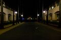  Path from Engineering Quad

Image Processing

With the captured scenes in hand, read out as the raw, mosaicked image, processing began by determining the orientation and patterning of the CFA on the sensor. This allows us to sample the mosaic at specific locations to extract the known color information as captured by each filter. From here, the demosaicking computations could begin in earnest.

Determining CFA orientation

In order to determine the patterning and orientation of the CFA, I looked at several regions, each of roughly uniform brightness and color. From there I could easily determine the white pixels, as they would have highest signal compared to the others. Given the known pattern of the pixels on each block of the CFA as supplied by the manufacturer, in addition to the known color of the region I were analyzing, I could correlate signal strengths in each of the non-white pixels to their expected color as R, G, or B. Making the assumption that the pattern orientation was constant throughout the sensor, I then used the expected filter arrangement to extract the mosaicked color channels, and ran simple linear interpolation on the RGB channels (ignoring white for now). If the colors in the resulting image appeared accurate relative to our reference image taken with a consumer camera (with some allowed discrepancy due to lack of white-balancing), I would know our determination was correct.

Alternatively, this process could be done with brute force by simply running simple linear interpolation given an assumed layout, and observing the results. However this would still involve human judgment, and due to the large size of the CFA, would take time, and perhaps produce results that only had a few pixels incorrect, leading to a possibility of choosing the wrong determined orientation. Therefore I believe our method was a good choice.

Abandoned methods

Several different methods toward demosaicking were attempted on this CFA. Due to the lack of information in the RGB channels (as a result of their sparse sampling of the scene as compared to the white channel), an initial attempt was made toward applying a compressive sensing framework to the problem [2]. Unfortunately this approach proved fruitless, as the sensing matrix could not be made to meet the restricted isometry property without modification of the imaging system. Work was then put toward attempting to design intelligent interpolation kernels to take into account cross-channel gradients (as inspired by Malvar et al. [3]), but due to the large size of the CFA period, this method was abandoned. Similarly, the large size of the CFA complicated the frequency domain characteristics of the mosaic, leading to a complex demultiplexing task for frequency-domain demosaicking. This, too, was therefore deemed implausible for the given timeframe of the experiment. Ultimately, more emphasis was placed on maximizing analysis regarding potential use-cases for the RGBC sensor. The primary use-case being extension of the usable dynamic range of the image.

Demosaicking

Images were first linearly interpolated on a per-channel basis. Given the high sampling rate of the white pixels relative to the RGB, the white channel then was used as an estimation of the luminance of the image. This is similar to other demosaicking methods on Bayer patterns where the green pixel is used as an estimate due to its similarly high sampling relative to the other pixels. The RGB interpolations are then combined into a lower-resolution RGB image, which is then transformed in luminance and chrominance space (YCbCr, specifically), through MATLAB's rgb2ycbcr function. I then extract the RGB-based low-resolution luminance map, and the chrominance channels are set aside to be reintegrated later.

Whenever possible, the luminance map from the white pixels should be used, as it contains the most signal and the highest resolution. However in regions were the white pixels are saturated, the luminance map from these pixels is unusable. It is at these points where I utilize the luminance map of the RGB image. I combine these luminance maps using very simple thresholding, with the edges of the replacement layer being low-passed in order to avoid sharp differences, and to ignore very small shadows. (This step currently requires tuning on a per-image basis to utilize the proper amounts of each luminance channel. In this proof-of-concept model, this is sufficient, but further work should lead to techniques where this parameter tuning is rendered unnecessary.)

It is important to note here that this process of combining the luminance maps is the key step of utilizing the wider HDR available to this CFA. I are in effect compressing the dynamic range, by bringing up values that would have been lost without the C pixel, and saturated values, choosing instead to utilize the relatively lower RGB values at those locations. The dark regions which are preserved by the C pixel are then displayed as closer to the bright regions than in actuality, resulting in a compressed high dynamic range.

The new merged luminance map is then combined with the chrominance from before, though indirectly. Rather than simply replace the luminance then apply a yCbCr to RGB transform (which would fail due to the interrelations of the luminance and chrominance levels), we instead scale the RGB channels by the ratio of the new luminance to the old luminance. This results in the channels receiving a boost luminance detail while also preserving any underlying colors that were present in low levels. If the signal were truly under the noise floor, the RGB channels would have roughly the same value, resulting in a grey value, but still granting detail where there previously was not any. This effect of bringing grey details out from below the noise floor is very similar to the effect produced in Interleaved Imaging as proposed by Parmar and Wandell [1].

The resulting image is then gamma-corrected using a gamma of 2.2, and color-corrected. The color-correction was performed using a rough form of white-balancing in which the Macbeth ColorChecker was isolated in the image, then pixel values at the grey squares were analyzed. Since the greys should be neutral where r = g = b, the global channels were normalized to achieve this relation in the grey regions. The weights required for normalization were found to be roughly the same throughout multiple scenes, so this normalization was used for color-correction on all images.

Results and discussion

Comparisons were done versus the pure RGB extrapolations without the white luminance map. This is important to remember when observing the dataset, as it means the comparison image will be relatively lacking in detail in comparison to the applied images. The important areas of comparison then are in the effects on contrast, discernable features, and color preservation in exceptionally dark areas. Observations in these areas are highlighted, and their results are notable.

Metric results such as PSNR and MSE are less applicable here due to their requirements of a pure reference for comparison. Since our method required capture of new data, and the only reference was from a consumer camera of different sensor type, this was not possible in this circumstance. With the known spectral sensitivity curves however, tests could be done on true, controlled HDR datasets to produce quantified results.

The RGB channels produced through linear interpolation are rather low-resolution as a result of the low sampling rate in the CFA. Since I rely primarily on the RGB channels solely for chrominance information in our technique however, this is not a prominent effect, as the human visual system is much more sensitive to changes in luminance than in chrominance. This low-pass effect on the chrominance is actually quite common, and is one of the core principles behind many compression applications.

This reality does come into play, however, in areas in which the white pixels have become oversaturated. In these areas, the more finely sampled white mosaic can no longer be used for the luminance channel, thus I are restricted to using only the luminance from the RGB pixels, more than halving our sample rate in those regions. This presents a troubling case for the CFA in its most ideal use case: that in which the RGB pixels are nearly saturated, allowing for maximal coverage of the DR of the scene with the RGB covering the bright regions and the white, the dark. Of course, this is not the final word for this use case. With more advanced methods of demosaicking low-rate sampled scenes, better performance could be expected in these regions.

Results with the night shots were not noteworthy. At the requisite exposure times, almost all objects of interest are well lit enough to the point of the clear pixel granting little extra. Since the DR of interest is not large, equivalent results could be found with a typical Bayer pattern. One possible advantage here is perhaps in shortening the requisite exposure time for such shots.

Unfortunately the presence of the white pixel is not a panacea for all circumstances. Most notably there are some scenes that possess too great a DR for the white pixels to capture the lowest signals while having the RGB pixels not saturating. Several of these cases emerged with our test images (the Memorial Church door scene is one example). While the RGBC CFA does increase the dynamic range acquisition capabilities over a standard RGB CFA, it cannot match the natural DR of some scenes.

Conclusion

In the ideal scenes, where the captured image possesses well-exposed RGB pixels that are unable to capture detail in certain dark regions within the range of the clear pixels, a notable improvement in SNR can be observed in regions of relative darkness. Local contrast in these regions is improved greatly, colors are more vivid, and details are preserved well as a result of the high sampling rate of the white pixels. These results present strong evidence toward usability of the RGBC CFA in HDR capture scenarios.

Results Gallery

• Result images with using C and without, some with artifacting to be ignored
• 

  1.5ms, without C

• 

  1.5ms, with C

• 

  1.5ms, crop, without

• 

  1.5ms, crop, with

• 

  0.72ms, without

• 

  0.72ms, with

• 

  1.31s, without

• 

  1.31s, with

• 

  1.31s, crop, without

• 

  1.31s, crop, with

• 

  300ms, without

• 

  300ms, crop, without

• 

  300ms, crop, with

• 

  100ms, without

• 

  100ms, with

• 

  100ms, crop, without

• 

  100ms, crop, with

• 

  100ms, without

• 

  100ms, with

• 

  100ms, crop, without

• 

  100ms, crop, with

• 

  2.5ms, without

• 

  2.5ms, with

• 

  2.5ms, crop, without

• 

  2.5ms, crop, with

• 

  2.5ms, without

• 

  2.5ms, with

• 

  2.5ms, crop, without

• 

  2.5ms, crop, with

References

[1] Parmar, Manu, and Brian A. Wandell. "Interleaved imaging: an imaging system design inspired by rod-cone vision." IS&T/SPIE Electronic Imaging. International Society for Optics and Photonics, 2009.

[2] Moghadam, Abdolreza Abdolhosseini, et al. "Compressive demosaicing."Multimedia Signal Processing (MMSP), 2010 IEEE International Workshop on. IEEE, 2010.

[3] Malvar, Henrique S., Li-wei He, and Ross Cutler. "High-quality linear interpolation for demosaicing of Bayer-patterned color images." Acoustics, Speech, and Signal Processing, 2004. Proceedings.(ICASSP'04). IEEE International Conference on. Vol. 3. IEEE, 2004.

[4] Rafinazari, Mina, and Eric Dubois. "Demosaicking algorithms for RGBW color filter arrays." Electronic Imaging 2016.20 (2016): 1-6.

Code

Code and data can be found here. Certain data concerning the CFA is not included due to restrictions on publication.