Fannjiang

Compressed Sensing in Astronomical Imaging

Introduction

Compressed sensing, which proposes the recovery of sparse signals from highly sub-Nyquist sampling, is a recent advancement in signal processing that has always intrigued me. Just as image compression schemes like JPEG have helped lighten expensive data storage and transmission, compressed sensing could reform the expensive data acquisition that is an element of many modern imaging systems. (Romberg 2008 gives a great introduction.) For my project, I did a simple implementation of compressed sensing for an imaging system used in astronomy, known as radio interferometry. Early in the literature of compressed sensing, radio interferometry was noted in Wiaux et al. 2009 and others as an ideal candidate for application, as it conforms to the two principles compressed sensing works by. The first is signal sparsity, where most of the signal's coefficients are zero or near-zero in some transform space; the second is incoherence of the measurement matrix, or a property known as the restricted isometry property, where (roughly speaking) the underdetermined measurement matrix has columns that are "nearly" orthogonal. The measurement matrix in radio interferometry is in essence the "partial Fourier ensemble" described in Donoho 2006, or "the collection of n × m matrices made by sampling n rows out of the m × m Fourier matrix". The partial Fourier ensemble was one of the first measurement matrices proven to work well for compressed sensing, as shown in Candès et al. 2006, which makes radio interferometry a natural candidate.

"Sampling n rows out of the m x m Fourier matrix" leaves open the question of which n rows, however. In radio interferometry, the set of rows is determined by the placement of the radio antennas in the antenna array. Random sampling has proven to be critical to much of compressed sensing theory, which clashes with the highly patterned arrays used in radio interferometry such as the prominent Very Large Array (VLA). Wenger et al. 2010 noted this clash, and ran a few numerical simulations to see whether a randomized array or the traditional patterned array would work better for compressed sensing. The authors report that the VLA's patterned array actually outperforms a uniform random array, which I thought was an interesting and somewhat counterintuitive result. So for my project, I ran similar numerical simulations, with some deviations from the paper:

• I incorporated the discrete cosine transform (DCT) covered in class to represent images sparsely, whereas Wenger et al. just took advantage of the fact that radio images tend to be sparse in the pixel domain.
• I used orthogonal matching pursuit (OMP), a greedy compressed sensing algorithm, whereas the original paper used SparseRI, a compressed sensing recovery scheme the authors designed specifically for radio interferometry.
• I compared the VLA to a random Gaussian array, as many of the massive up-and-coming interferometers like the Atacama Large Millimetre/submillimetre Array (ALMA) (which celebrated its inauguration this month!) and Square Kilometre Array (SKA) seem to be centrally condensed as well as randomized, whereas the paper compared the VLA to a uniform random array.

To simulate signals from astronomical radio sources, I just took images the VLA has published on their online image gallery [8] and vectorized them. If the radio source is thought of of as an array of point sources, then the brightness value of each pixel in the image represents the intensity of each point source.

Background

Imaging in Radio Astronomy

Interferometry is the definitive imaging tool of radio astronomy, allowing us to image finely structured radio sources such as galaxies, nebulas, and supernova remnants by using an array of many antennas to emulate a single lens. The aperture of the array is the greatest pairwise distance between antennas—which, at several kilometers for interferometers like the VLA in New Mexico, gives us far higher imaging resolution than a single lens could.

The Very Large Array, which uses 27 antennas.

• 

  Radio emission of Orion Nebula, imaged by the VLA. Courtesy of NRAO/AUI and F. Yusef-Zadeh.

• 

  Radio emission of the galaxy 3C353, imaged by the VLA. Courtesy of NRAO/AUI, Mark R. Swain, Alan H. Bridle, and Stefi A. Baum.

• 

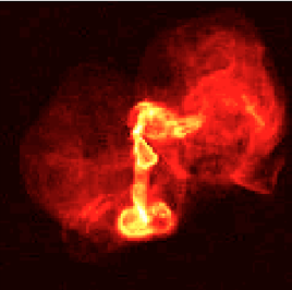
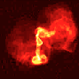
  Radio emission of the G21.5-0.9 supernova remnants, imaged by the VLA. Courtesy of NRAO/AUI and M. Bietenholz.

Radio interferometry works by measuring the visibility function, or the interference fringes of the radio signal, at every pair of antennas in the array. The van Cittert-Zernike theorem gives the visibility function, as measured by one pair of antennas in the array, over the viewing window of the sky P as

$V(\mathbf {b} )=\int \limits _{\mathit {P}}I(\mathbf {p} )e^{-2\pi i\mathbf {b} \cdot \mathbf {p} }{\mathit {d}}\mathbf {p} ,$

where $\mathbf {b}$ is the displacement vector between the two antennas, called the baseline, and $I(\mathbf {p} )$ is the intensity of the radiation from direction $\mathbf {p}$. Assuming a small field of view, such that the object $I(\mathbf {p} )$ lives on the plane instead of the sphere, the visibility measurements can be approximated as

$\mathbf {V} \approx (\Delta \mathbf {p} )^{2}\sum _{k}\mathbf {I} (\mathbf {p} _{k})e^{-2\pi i\mathbf {b} \cdot \mathbf {p} _{k}}$.

In effect, the array samples the two-dimensional Fourier transform of the spatial intensity distribution $I(\mathbf {p} )$ of the radio source. It collects one Fourier coefficient with each baseline, or each pair of antennas. Ideally, if we thoroughly sample the Fourier plane, we can then invert the transform to reconstruct $I(\mathbf {p} )$, the image of the radio source. However, the data acquisition quickly gets expensive, as we need to capture one Fourier coefficient per desired pixel in the image. The need to capture so much data has motivated a new generation of ambitious interferometers, including the ALMA, which will use 66 antennas, and the Square Kilometre Array (SKA), which will use several thousand antennas to probe the Fourier plane. Meanwhile, smaller interferometers like the 27-antenna VLA must sample over an extended period of time.

Despite such efforts, there are always irregular holes on the Fourier plane where sampling of the visibility function is thin or simply nonexistent. This data deficiency is currently managed by filling in zeros for unknown visibility values, and applying deconvolution algorithms such as CLEAN to the resulting “dirty images”. However, is it necessary to collect so much data in the first place?

Among imaging's most promising developments in recent years is the theory of compressed sensing (CS), which has shown that the information of a signal can be preserved even when sampling does not fulfill the fundamental Nyquist rate. The theory revolves around a priori knowledge that the signal is sparse or compressible in some basis, in which case its information naturally resides in a relatively small number of coefficients. Instead of directly sampling the signal, whereby full sampling would be inevitable in finding every non-zero or significant coefficient, CS allows us to compute just a few inner products of the signal along measurement vectors of certain favorable characteristics. (Here, the measurement vectors are the Fourier-like measurement vectors described by the van Cittert-Zernike theorem above.) The novelty of CS over image compression is that it takes advantage of image compressibility to lighten data acquisition, not just data storage.

Compressed Sensing

Consider a signal $\mathbf {x}$ in $\mathbb {R} ^{N}$, which has a sparse representation $\mathbf {s}$ with the columns of an ${\mathit {N}}\times {\mathit {N}}$ basis matrix $\Psi$, such that $\mathbf {x} =\Psi \mathbf {s}$. Given that $\mathbf {s}$ is ${\mathit {S}}$-sparse, meaning it has only ${\mathit {S}}\ll {\mathit {N}}$ non-zero components (or, more generally, given that $\mathbf {s}$ is ${\mathit {S}}$-compressible and has only ${\mathit {S}}\ll {\mathit {N}}$ "significant components") and given measurement vectors of certain favorable characteristics, CS proposes that we should not have to take the complete set of ${\mathit {N}}$ inner-product measurements to recover the signal. If $\Theta$ is an ${\mathit {M}}\times {\mathit {N}}$ matrix whose ${\mathit {M}}<{\mathit {N}}$ rows are the measurement vectors, then CS aims to invert the underdetermined linear system $\mathbf {y} =\Theta \Psi \mathbf {s} =\Phi \mathbf {s}$, where $\mathbf {y}$ is a vector of the ${\mathit {M}}<{\mathit {N}}$ measurements of $\mathbf {x}$ and we call $\Phi$ the measurement matrix.

If $\mathbf {s}$ is sparse, intuitively we should seek a sparse solution to the inverse problem. Indeed, in the absence of noise $\mathbf {s}$ is the sparsest solution, i.e., the $\mathbf {\hat {s}}$ subject to $\mathbf {y} =\Phi \mathbf {\hat {s}}$ that has the least number of non-zero components. A direct search for this solution, however, is computationally intractable. Given $\Phi$ of favorable characteristics (described below), an $\ell _{1}$-minimization problem can be solved instead, such that we search for the solution $\mathbf {\hat {s}}$ with the smallest $\ell _{1}$-norm, or sum of the absolute values of the coefficients. CS recovery schemes also include greedy algorithms to solve a similar "$\ell _{0}$-minimization" problem, such as OMP, which I used (mostly because it runs much faster than basis pursuit and LASSO, the classic $\ell _{1}$-minimization methods).

Recovering $\mathbf {x}$ requires that the measurement matrix $\Phi =\Theta \Psi$ does not corrupt or lose key features of $\mathbf {s}$ in mapping higher-dimension $\mathbf {s}$ to the lower-dimension $\mathbf {y}$. One simple and intuitive measure of the information content of $\mathbf {s}$ is its Euclidean norm. So we would hope that $\Phi$ nearly preserves the Euclidean norm of $\mathbf {s}$, which implies that every possible subset of ${\mathit {S}}$ columns of $\Phi$ is approximately orthonormal. (A rigorous formulation of this quality is known as the restricted isometry property, but unfortunately it cannot be checked empirically: checking every ${\mathit {S}}$-combination of columns of $\Phi$ for near-orthogonality is a combinatorial process and NP-hard.)

In radio interferometry, $\Theta$ is given by the van Cittert-Zernike theorem to be a partial Fourier ensemble. For my project, I used the DCT matrix as $\Psi$. Due to the role of the antenna array in selecting the rows of $\Theta$, the array plays a key role in designing an incoherent measurement matrix $\Phi$. Understanding what arrays are best for CS, as Wenger et al. 2010 explores, is therefore an important step before it can be used in radio interferometry in practice.

The Sparsifying Basis: DCT

The DCT, which was used in the original JPEG compression scheme, divides an image into 8-by-8 pixel blocks and calculates the following transform coefficients for each block:

$F(u,v)={\frac {C(u)C(v)}{4}}\sum _{x=0}^{7}\sum _{x=0}^{7}f(x,y)cos({\frac {2x+1}{16}}u\pi )cos({\frac {2y+1}{16}}v\pi )$ where $C(u)={\frac {1}{\sqrt {2}}}$ when $u=0$ and $C(u)=1$ otherwise; and $C(v)={\frac {1}{\sqrt {2}}}$ when $v=0$ and $C(v)=1$ otherwise.

Methods

Software

All of my simulated image reconstructions were done in MATLAB.

Orthogonal Matching Pursuit

I used the following CS recovery algorithm, described in Tropp and Gilbert 2007. OMP iteratively searches for the sparsest solution in the infinite solution space. In each iteration, it uses a greedy approach to find the brightest remaining pixel, corresponding to the column of the measurement matrix that has the highest coherence with the residual data. It then projects the data onto the span of all the columns selected so far to update the image reconstruction, and updates the residual. This process of selecting columns, projecting the data, and updating the residual continues until the residual falls below some threshold. I set the threshold to be 1% of the Euclidean norm of image.

• 

  The OMP algorithm, as described in Tropp and Gilbert 2007 [1].

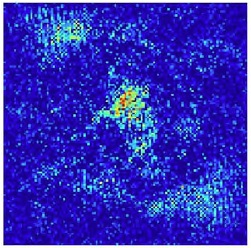
Array Models

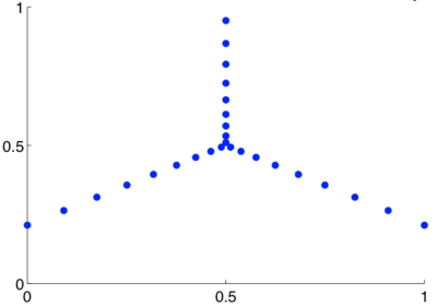
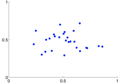
The VLA's 27 antenna coordinates are published in the VLA Green Book, and are plotted below. An array measures one Fourier coefficient with each pair of antennas, or baseline, so the set of baselines is also plotted. The baselines give the Fourier plane sampling of the array.

• 

  VLA antenna configuration. Calculated from the polar coordinates published in the VLA Green Book.

• 

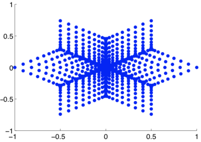  VLA baselines on the Fourier plane. Calculated by finding the displacement vectors between all pairs of antennas in the array.

I wanted to compare the VLA to modern massive interferometers like the just-inaugurated ALMA and the unfinished SKA, which is set to start observations in the 2020s:

• 

  ALMA antennas [2].

• 

  Artist's rendition of the planned SKA antennas [3].

I could not find published coordinates of the ALMA antennas, or the planned coordinates of the SKA antennas. Given their centrally condensed and randomized nature, I modeled them with a random Gaussian distribution of 27 antennas (since the VLA has 27 antennas). Boone 2002 notes that today's radio astronomy community believes a Gaussian sampling of the Fourier plane to be ideal, so this model should be suitable:

• 

  Random Gaussian distribution of antennas, which I used to model today's prototypical array (e.g. the ALMA and the SKA) in my simulations.

• 

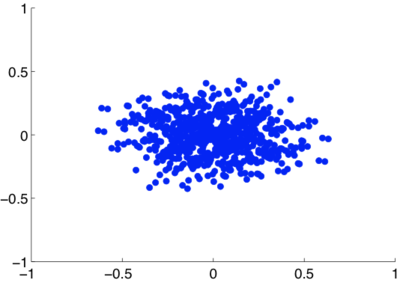  Baselines of a random Gaussian array on the Fourier plane. Calculated by finding the displacement vectors between all pairs of antennas in the array.

Test Images

I used the following test images, all from the VLA's beautiful online image gallery, for my imaging simulations.

• 

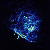
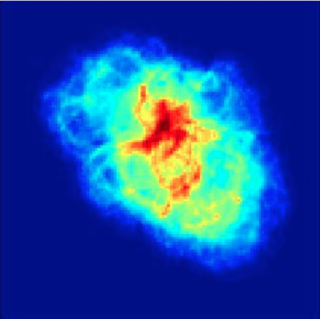
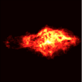
  Radio image of the Crab Nebula [4]. Courtesy of NRAO/AUI and M. Bietenholz.

• 

  Radio image of the Cassiopeia A supernova remnants [5]. Courtesy of NRAO/AUI.

• 

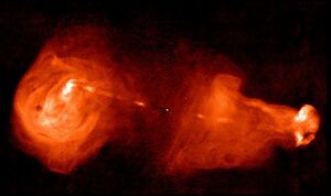
  Radio image of the galaxy M87 [6]. Courtesy of NRAO/AUI and F.N. Owen, J.A. Eilek, and N.E. Kassim.

• 

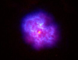
  Radio image of the galaxy 3C58 [7]. Courtesy of NRAO/AUI and M. Bietenholz.

Protocol

• Calculate two versions of the measurement matrix $\Theta$ using the formula given by the van Cittert-Zernike theorem, one with the VLA and one with a random Gaussian array. I roughly eyeballed the sparsity of the images, and took 1/3 the number of measurements traditionally needed for each image. For instance, for a 200 x 200 = 40,000-pixel image, I used a measurement matrix with 40,000 / 3 $\approx$ 16,000 rows, instead of the full 40,000 rows.
• Calculate the DCT matrix for the sparsifying matrix $\Psi$.
• Calculate $\Phi =\Theta \times \Psi$.

For each test image:

• Convert the image into a linear vector, representing $\mathbf {I} (\mathbf {p} _{k})$. I also further pixelized the original images: I used a 120-by-120 pixel version of the Crab Nebula image, a 200-by-200 pixel version of the Cassiopeia A image, a 120-by-120 pixel version of the M87 image, and a 160-by-160 version of the 3C58 image, so that MATLAB could process the image reconstructions within reasonable time (several hours).
• Calculate the simulated measurements $\mathbf {V} (\mathbf {b} )$ through the multiplication $\Phi \times \mathbf {I} (\mathbf {p} _{k})$.
• For each version of the measurement matrix $\Phi$, run OMP on $\mathbf {V} (\mathbf {b} )$ to recover the DCT coefficients of $\mathbf {I} (\mathbf {p} _{k})$.
• Multiply the recovered DCT coefficients by the DCT matrix $\Psi$ to reconstruct the image.
• For each version of the measurement matrix $\Phi$, calculate the relative error between the reconstructed image $\mathbf {\hat {I}} (\mathbf {p} _{k})$and the original image $\mathbf {I} (\mathbf {p} _{k})$: $RE={\frac {||\mathbf {\hat {I}} (\mathbf {p} _{k})-\mathbf {I} (\mathbf {p} _{k})||^{2}}{||\mathbf {I} (\mathbf {p} _{k})||^{2}}}$.

Results

Below are the image reconstructions resulting from the protocol described above.

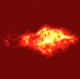
Image of the Crab Nebula

• 

  120-by-120 pixel radio image of the Crab Nebula.

• 

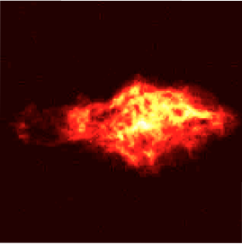
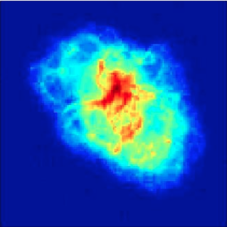  OMP reconstruction using the random Gaussian array. RE = 3.78%.

• 

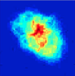  OMP reconstruction using the VLA configuration. RE = 7.52%.

The random Gaussian array clearly gives a more accurate reconstruction, while there are distinct blocking artifacts in the VLA reconstruction.

Image of the Cassiopeia A Supernova Remnants

• 

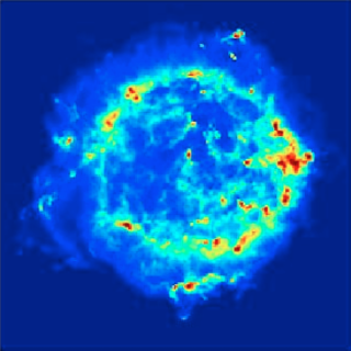  200-by-200 pixel radio image of the Cassiopeia A supernova remnants.

• 

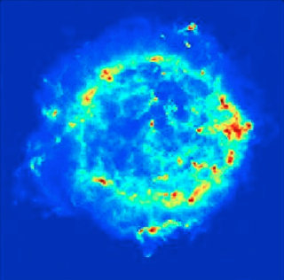  OMP reconstruction using the random Gaussian array. RE = 1.19%.

• 

  OMP reconstruction using the VLA configuration. RE = 0.33%.

Note the blocking artifacts in the VLA reconstruction.

Image of the Galaxy M87

• 

  120-by-120 pixel radio image of the galaxy M87.

• 

  OMP reconstruction using the random Gaussian array. RE = 0.20%.

• 

  OMP reconstruction using the VLA configuration. RE = 0.90%.

Note, again, the blocking artifacts in the VLA reconstruction.

Image of the Galaxy 3C58

• 

  160-by-160 pixel radio image of the galaxy 3C58.

• 

  OMP reconstruction using the random Gaussian array. RE = 1.37%.

• 

  OMP reconstruction using the VLA configuration. RE = 0.28%.

The patterned VLA configuration consistently causes blocking artifacts in the reconstructions. For these images, the dominant DCT coefficients in each block are typically the low-frequency coefficients. Therefore, when too few DCT coefficients are recovered by OMP, the missing coefficients (typically the high-frequency ones) create breaks in features that should span the blocks continuously. It appears that the patterned VLA configuration aggravates this phenomenon, while the random Gaussian array gives much more accurate reconstructions without blocking artifacts.

DCT versus the Pixel Basis

As CS revolves around the sparsity or compressibility of signals, one cannot take full advantage of CS without finding an optimal sparse representation of the signal. To highlight the advantage of using the DCT as a sparsifying basis instead of the pixel basis, as Wenger et al. 2010 did, I ran OMP on the simulated measurements of the Crab Nebula using the pixel basis. I simply set the sparsity matrix $\Psi$ to the identity matrix, instead of the DCT matrix.

• 

  120-by-120 pixel radio image of the Crab Nebula.

• 

  OMP reconstruction using the random Gaussian array and the DCT as the sparsifying basis.

• 

  OMP reconstruction using the random Gaussian array and the pixel basis.

Given the same set of measurements, the pixel basis gives a disastrous reconstruction, barely recovering enough pixels to confirm the nebula's existence. Natural images like these are typically far sparser and far more compressible in the DCT basis than in the natural pixel basis, which is critical to successful CS.

Conclusions

My imaging simulations confirmed that CS can be successfully applied to radio interferometry, as the literature has suggested. For each image, I took only 1/3 the number of measurements traditionally needed—and it may be possible to take less, as I was simply eyeballing the sparsity of the images—and yet OMP was able to reconstruct images with surprisingly low relative error.

In all my simulations, the random Gaussian array provides far more accurate reconstructions than the patterned VLA configuration. Though this result aligns with the principle of random sampling predominant in CS theory, it contradicts the results of Wenger et al. 2010, which reported that the patterned VLA configuration gave more accurate CS reconstructions. There are several possible explanations for this deviation: the first is that the paper compared the VLA to a uniform random distribution of antennas, not a centrally condensed distribution such as a Gaussian. Though both a uniform random array and random Gaussian array have the randomized nature that the VLA lacks, the difference between uniform and centrally condensed coverage of the Fourier plane may have been critical. Secondly, Wenger et al. used a CS recovery scheme they developed themselves, called SparseRI. The paper did not describe the nature of the recovery scheme, though it does appear to be specialized for radio interferometry, rather than a general, widely used CS framework such as OMP. Thirdly, the paper did not use a sparsifying basis like the DCT and ran the reconstructions in the pixel basis. These differences in our methods may explain why Wenger et al. preferred the patterned VLA configuration for CS,while my simulations preferred a random Gaussian array.

Future Work

The deviations between our simulations provide many ideas for future work. Finding an optimal sparsifying basis for radio images is particularly important, and multiresolution schemes such as wavelet bases can be considered. Radio interferometry in general has not been practiced outside of the pixel basis, and these simulations highlight the important of doing so before CS can be applied. The CS recovery algorithm is also a key variable: I used the OMP largely because it is much more computationally efficient than $\ell _{1}$-minimization approaches like basis pursuit and LASSO, but these may respond to antenna arrays differently. As we look to deal with new floods of data from massive arrays, including the ALMA and the SKA, optimizing these factors for CS in radio interferometry will become more and more important.

References

Boone, F. Astronomy & Astrophysics, 386: 1160 - 1171, 2002. [9]

Candès, E., Romberg, J., and Tao, T. Robust uncertainty principles: Exact signal reconstruction from highly incomplete frequency information. IEEE Trans. Inform. Theory, 52:489 - 509, 2006. [10]

Donoho, D.L. Compressed sensing. IEEE Trans. Inform. Theory, 52:1289 -1306, 2006. [11]

Romberg, J. Imaging via compressive sampling. IEEE Signal Proc. Mag., 25:14 - 20, 2008. [12]

Tropp, J. and Gilbert, A. Signal recovery from random measurements via orthogonal matching pursuit. IEEE Trans. on Information Theory, 53: 4655 - 4666, 2007. [13]

Wenger, S., Darabi, S., Sen, P., Glassmeier, K., and Magnor, M. Compressed sensing for aperture synthesis imaging. Proc. IEEE International Conf. on Imag. Proc, 1381, 2010. [14]

Wiaux, Y., Jacques, L., Puy, G., Scaife, A.M.M., and Vandergheynst, P. Compressed sensing imaging techniques for radio interferometry. Monthly Notices of the Royal Astr. Soc., 395:1733 - 1742, 2009. [15]

Appendix

MATLAB code: File:MATLABCode.zip

Link to a PostScript-format download of the VLA Green Book, which publishes the polar coordinates of their antennas in Chapter 1: [16]

Links to the test images, taken from the VLA's website:

Radio image of the Crab Nebula: [17]

Radio image of the Cassiopeia A supernova remnants: [18]

Radio image of the galaxy M87: [19]

Radio image of the galaxy 3C58: [20]