Impact of Camera Characteristics on DNN Model Inference Performance

Introduction

In the current age of the AI revolution, there are numerous image recognition applications reliant on pre-trained deep neural networks (DNNs). Images used in training the DNNs for these application may be captured by a variety of users, cameras, environments, etc. Same holds for test-time inference which begs the question: how may the image characteristics impact the DNN performance? In this project, using ISET AI CameraDesigner, we experiment with generating images with different camera characteristics and evaluate several pre-trained DNN models on their inference accuracy. Observations are made on the impact of image quality on predictions.

Background

F/#

The ratio of the aperture diameter to focal length. It is an indicator of the amount of light going through the lens.
$N=f/D$
N: F/# (F-Number)
f: Focal Length (m)
D: Aperture Diameter (m)

Focal Length

Measured in millimeters, it is the distance between the optical center and the sensor plane. It correlates with how strongly the system converges or diverges light.

Exposure Time

Measured in seconds, it indicates the duration of the light collection by the camera sensor.

ISET AI Camera Designer

• Build Camera subsystems; Optics, Sensor, and IP.
• Use a collection of images.
• Generate Images from the original Images with the Camera Design.
• Evaluates Original Images vs Generated Images on different pre-trained DNNs.
  • Scores are based on the classification match (top-1) of the original and generated images.

ImageNet Dataset

• Used in training all DNN models used
• 1000 classes/categories
• 1,281,167 training images 
• 50,000 validation images 
• 100,000 test images 

DNN Architectures

• Pre-trained on ImageNet dataset and available in Matlab
• Chosen for smaller footprint targeting embedded applications
• All Convolutional Neural Networks (CNNs)
• Output a predicted class using probability distribution from softmax
• Increase representational power by successive feature space reduction and expansion.

DNNs Architectures

DNN Architecture	Depth	Size	Parameters (Millions)	Image Input Size
GoogleNet	22	27 MB	7.0	224-by-224
SqueezeNet	18	5.2 MB	1.24	227-by-227
ShuffleNet	50	5.4 MB	1.4	224-by-224
MobileNetV2	53	13 MB	3.5	224-by-224
EfficientNetB0	85	20 MB	5.3	224-by-224

​ GoogleNet: It was introduced in 2014. It is an inception module with 1x1 convolutions used to reduce the parameter space enabling increased depth.

SqueezeNet: It was introduced in 2016. It has a fire module made from squeeze convolution layer (1x1 filters) and expand convolution layer (combination of 1x1 and 3x3); force distillation of information.

ShuffleNet: It was introduced in 2017. The architecture use pointwise group convolution to reduce computation cost and channel shuffle to help information flow across feature channels.

MobileNetV2: It was introduced in 2018. The architecture consists of depthwise separable convolutions to reduce the complexity cost and model size from v1.

EfficientNetB0: It was introduced in 2019 and discovered by Neural Architecture Search (NAS) using a principled compound scaling method to uniformly scale network width, depth, and resolution with a set of fixed scaling coefficients​.

Methods

MATLAB-based ISET AI Camera Designer was the principal tool in generating images with different camera characteristics. Different DNN models and camera characteristics were used to measure the mean classification accuracy of the Beagle category (a total of 196 images) and analyze them.

ISET AI Camera Designer

• 

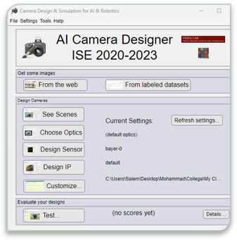  Picture 1: ISET AI Camera Designer Application

• Uses a collection of images provided by the user.
  
• Simulates camera module effects over different subsystems: Optics, Sensor, and ISP.
  
• Applies chosen effects to the provided images generating new images.
  
• Evaluates original and generated images on selected pre-trained DNNs. By default scores are based on the classification match between the original and generated images as opposed to a provided ground-truth label. In this project we provided the fixed label ("Beagle" category) to evaluate both original and generated image classification.
  

Experiments

In this project, we tweaked the camera characteristics by incorporating a combination of parameters in the camera subsystems such as Optics and Image Sensor. Our approach involved conducting multiple experiments to thoroughly investigate the effect of the different camera characteristics on the DNN models classification.

The combination of data used in each of the experiments is as follows:

F/# - Focal Length Combination

In this combination experiment, we assessed classification accuracy based on the presence of the correct label within the top predicted class. Data and Images were generated with a combination of f-numbers and focal lengths to explore if there are any interesting relations. The combination were used in the data collection are as follows which provide 40 deferent datasets:

F/#: f/1.0, f/1.4, f/2, f/4, f/5.6, f/8, f/11, f/16, f/22, f/32

Focal Lengths used for each of F/#: 15, 20, 35, 50 mm

Exposure Time

In this experiment, we assessed classification accuracy based on the presence of the correct label within the top five predicted classes which more tolerant than the F/# and Focal Length combination experiment. Also, the data was collected by only modifying the exposure time. The exposure times were used in the data collection are as follows:

Exposure Times: 5, 10, 20, 40, 80 milliseconds.

Read Noise

In this experiment, the classification accuracy was assessed as same as the Exposure Time based on the top five predicted classes. The images were generated with the default settings of the Camera Designer App. However, we only modified the read noise of the camera sensor. The read noise values that were used in the data collection are as follows:

Read Noise: 1, 10, 50, 100, 200 mV

Results

• 

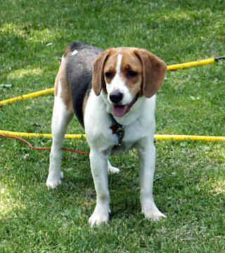  Picture 2: Beagle Original Image from Image Net

In the data collection and generating images, we used the Beagle Category from the ImageNet dataset. In this write-up, we will use Picture 2 as the base image and display the effect of the Camera parameters on it.

F/# and Focal Length

• 

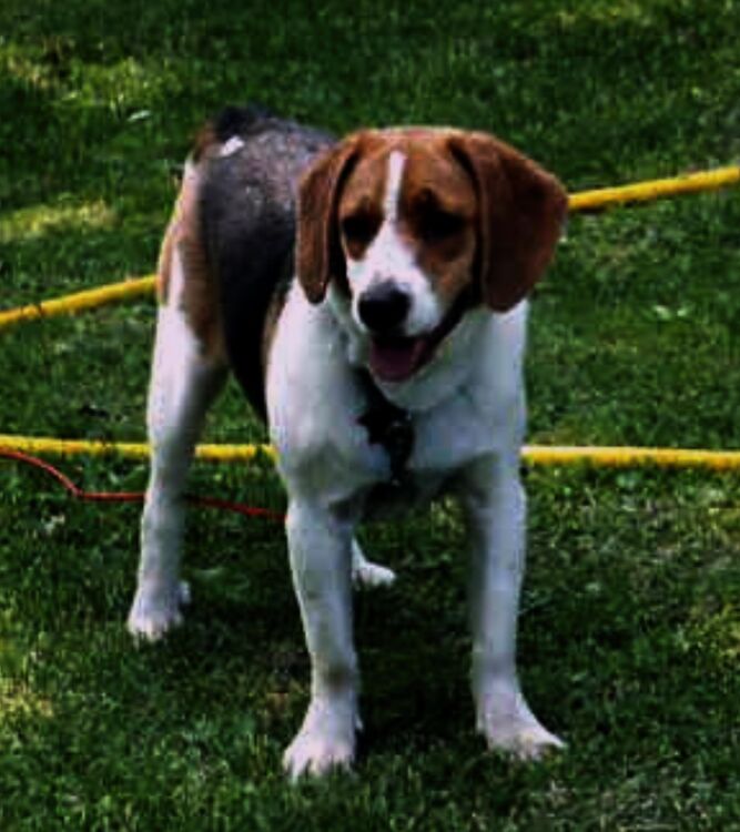
  Picture 3: Beagle Image with F/4 and Focal length of 15 mm

• 

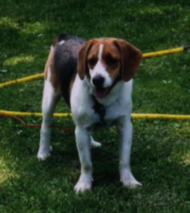
  Picture 4: Beagle Image with F/4 and Focal length of 50 mm

• 

  Picture 5: Beagle Image with F/32 and Focal length of 15 mm

In F/# and Focal Length experiment, the modification of the parameters cause some blurriness and zoom effects on the base images as shown in the Pictures 3, 4 and 5. SqueezeNet and ShuffleNet performed poorly when compared to the other architectures because these 2 have the smallest parameter count limiting their expressivity; representational power.

• 

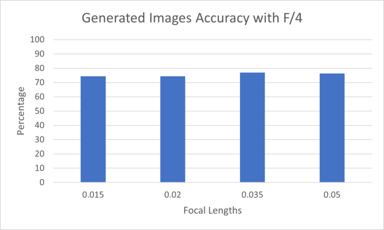  Figure 1: Generated Images Accuracy for the different Focal Lengths with F/4 evaluated on EfficientNetB0

• 

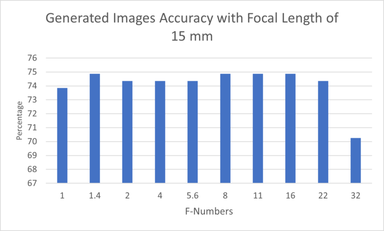  Figure 2: Generated Images Accuracy for the different F-Numbers with Focal Length of 15 mm evaluated on EfficientNetB0

• 

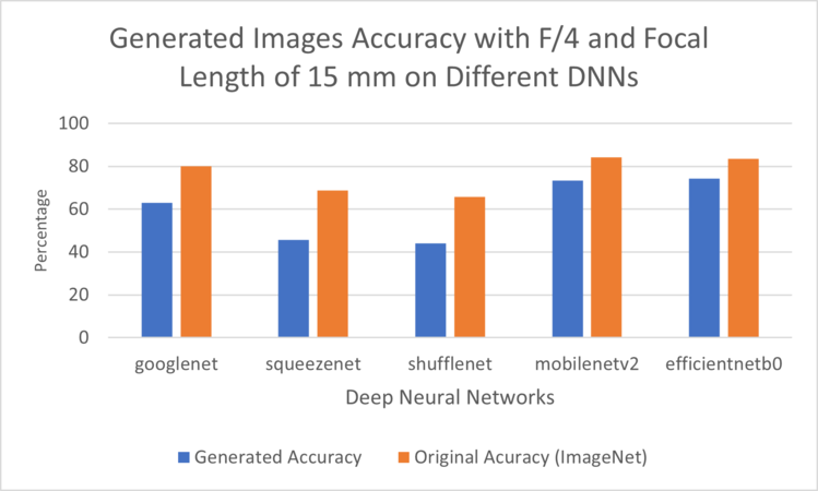  Figure 3: Generated Images Accuracy for F/4 and Focal Length of 15 mm Exposure Time evaluated on deferent DNNs

In Figure 1, the chart does not show impact on the classification when the focal length is modified. Similarly, when the Focal length is fixed and the F-number is change. However, only when the F-Number is set to F/32, the image is blurry causing decrease in the classification accuracy as shown in Figure 2.

• 

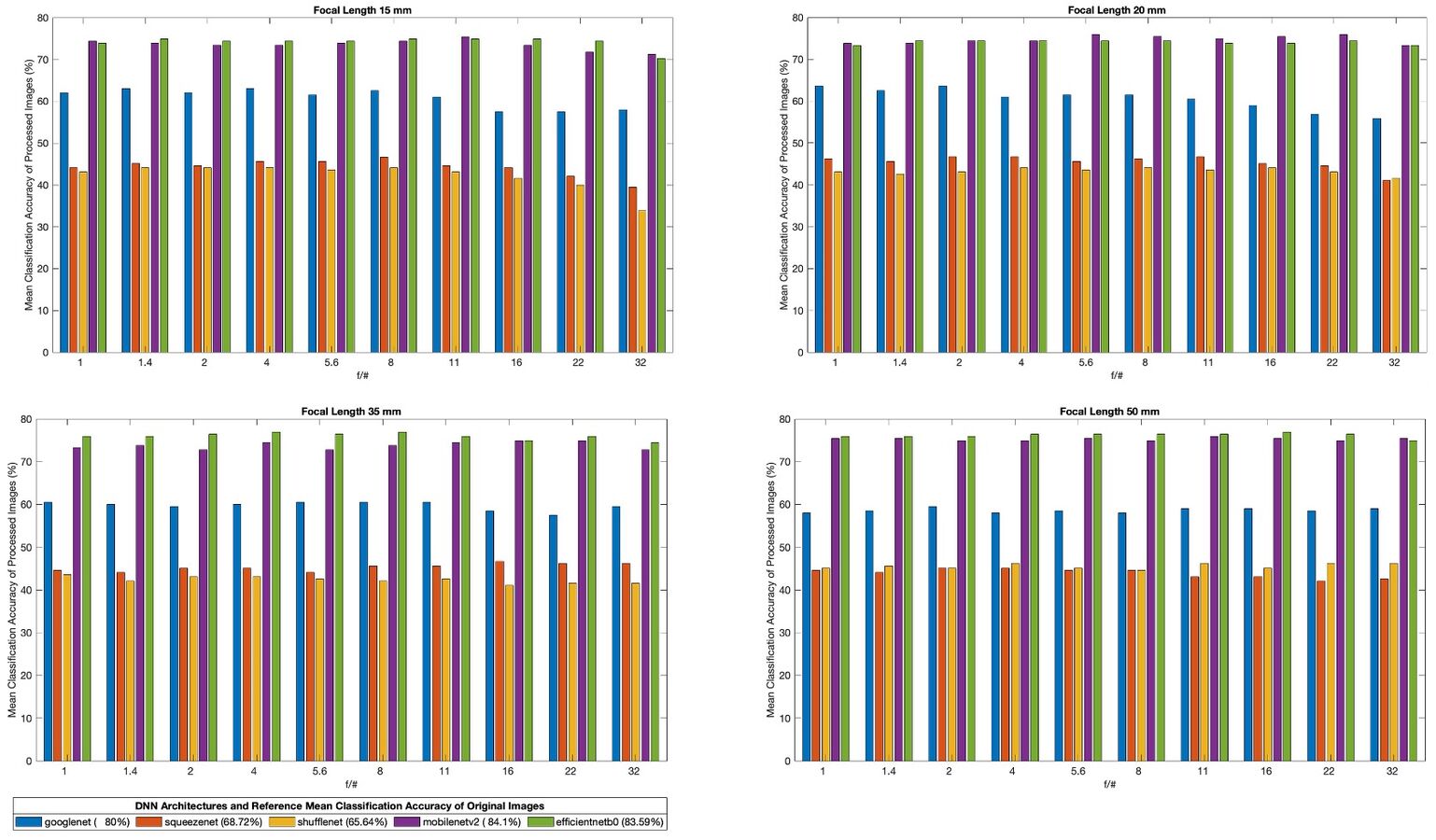  Comparative chart of combined f/# and focal length effects over all DNN models.

In the comparative chart of combined f/# and focal length effects over all DNNs using generated images, it can be seen that

• squeezenet and shufflenet perform poorly when compared to the other architectures; these 2 have the smallest parameter count limiting their representational power
• despite having the largest parameter count, googlenet performs worse than mobilenetv2 and efficientnetb0
• some architectures see improvements when increasing the f/# (e.g, squeezenet at focal length 35) while others see degradation in performance (e.g., shufflenet at focal length 35); both see degradation at focal length 15 while increasing f/#

Note that the included legend provides reference performance of the original images. All generated images show decreased performance relative to the original images likely due to a combination of image degradation and domain gap between training and test images.

• 

  GoogleNet: comparative chart of combined f/# and focal length effects.

• 

  SqueezeNet: comparative chart of combined f/# and focal length effects.

• 

  ShuffleNet: comparative chart of combined f/# and focal length effects.

• 

  MobileNetV2: comparative chart of combined f/# and focal length effects.

• 

  EfficientNetB0: comparative chart of combined f/# and focal length effects.

From the per-DNN comparative chart of combined f/# and focal lengths effects the following can be noted:

• EfficientNetB0 shows degradation at increased f/# (32) while improving with focal length increase.
• GoogleNet shows a degradation trend over the f/# sweep
• MobileNet shows overall robust performance across the sweeps with a slight deterioration at f/# 32 at lower focal lengths
• ShuffleNet shows a notable improvement at highest focal length across the f/# sweep
• SqueezeNet shows improvement for focal length 35 over the f/# sweep though degradation at the other focal lengths

Exposure Time

• 

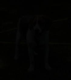  Picture 6: Beagle Image with 10 milliseconds exposure time

• 

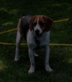  Picture 7: Beagle Image with 80 milliseconds exposure time

In the Exposure Time experiment, the images clearly reveal the impact of exposure time. A direct relationship is observed: as exposure time increases, the images become brighter, and conversely, they become darker.

• 

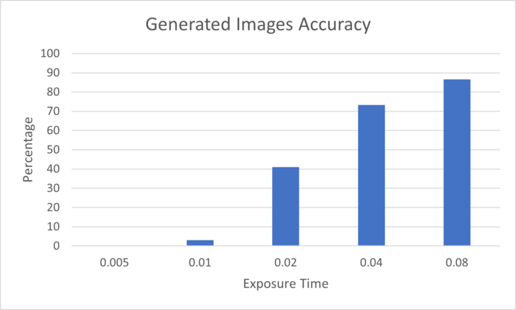  Figure 4: Generated Images Accuracy for the different Exposure Times evaluated on EfficientNetB0

• 

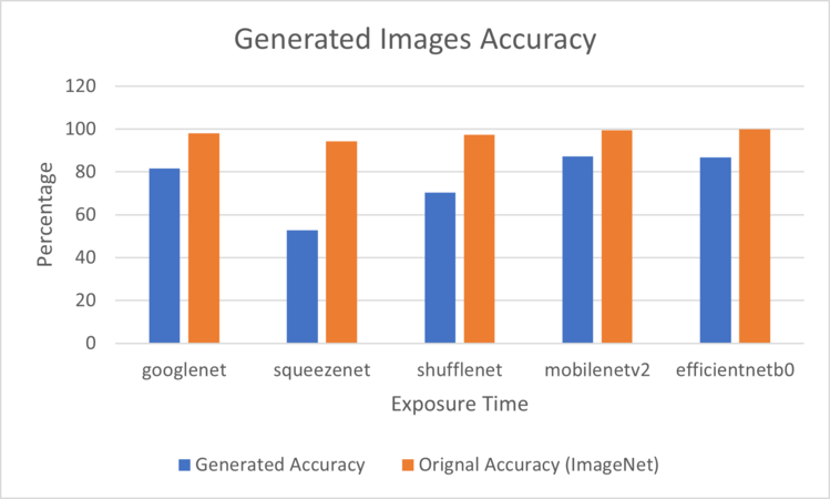  Figure 5: Generated Images Accuracy for 80 milliseconds Exposure Time evaluated on deferent DNNs

In Figure 4, the chart illustrates the impact of the exposure time on the classification accuracy. The greater the exposure time, the better the classification accuracy since the images are clearer and sharper. Also, it is noticeable among the various deep neural networks (DNNs) employed to assess the images, the performance of the SqueezeNet DNN was the worst with a 52.8% accuracy, as shown in Figure 5, while the MobileNetV2 archived the best accuracy with 87.2%.

Read Noise

• 

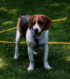  Picture 8: Beagle Image with 1 mV Read Noise

• 

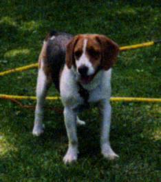  Picture 9: Beagle Image with 200 mV Read Noise

In the Read Noise experiment, there is a subtle dissimilarity between the images, which may not be immediately apparent. The image on the right exhibits more noise, resulting in a loss of some finer details.

• 

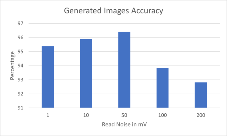  Figure 6: Generated Images Accuracy for the different Read Noises evaluated on EfficientNetB0

• 

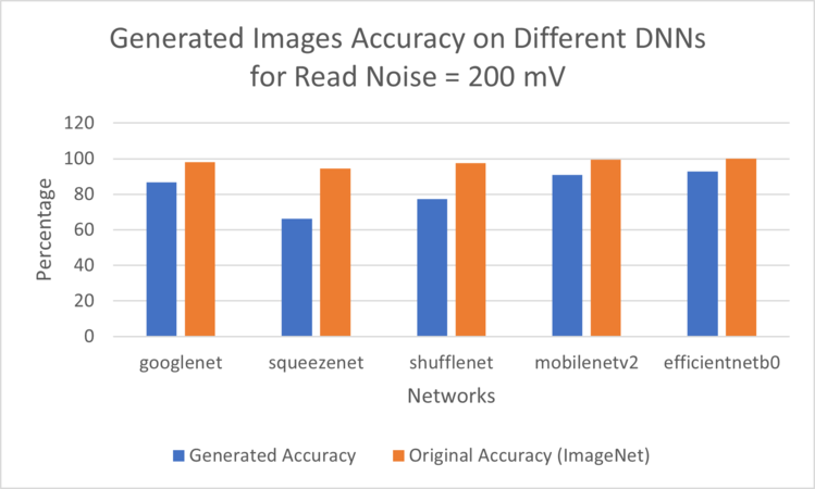  Figure 7: Generated Images Accuracy for 200 mV Read Noise evaluated on deferent DNNs

In Figure 6, the chart depicts a decline in classification accuracy corresponding to an increase in read noise. While the decrease may not be statistically significant, it is evident that the accuracy tends to decline with an increase in read noise. Notably, SqueezeNet exhibited the worst performance with a classification accuracy of 66.2%, while MobileNetV2 and EfficientNetB0 demonstrated the highest classification accuracies in this experiment.

Conclusions

• DNN model performance is impacted by camera parameters
• Empirical iterative discovery process to determine impact direction and magnitude
• Camera parameters’ adjustments can be applied at training time either to restrict or widen the data distribution depending on application
  • Restrict to target a smaller model parameter space (more constrained application)
  • Widen to generalize better (less constrained application)
• At inference time they can bring an out-of-distribution example into in-distribution

References

• J. Deng, W. Dong, R. Socher, L. -J. Li, Kai Li and Li Fei-Fei, "ImageNet: A large-scale hierarchical image database," 2009 IEEE Conference on Computer Vision and Pattern Recognition, Miami, FL, USA, 2009, pp. 248-255, doi: 10.1109/CVPR.2009.5206848.

• C. Szegedy et al., "Going deeper with convolutions," 2015 IEEE Conference on Computer Vision and Pattern Recognition (CVPR), Boston, MA, USA, 2015, pp. 1-9, doi: 10.1109/CVPR.2015.7298594.

• Iandola, F.N., Moskewicz, M.W., Ashraf, K., Han, S., Dally, W.J., & Keutzer, K. (2016). SqueezeNet: AlexNet-level accuracy with 50x fewer parameters and <1MB model size. ArXiv, abs/1602.07360.

• Zhang, X., Zhou, X., Lin, M., & Sun, J. (2017). ShuffleNet: An Extremely Efficient Convolutional Neural Network for Mobile Devices. 2018 IEEE/CVF Conference on Computer Vision and Pattern Recognition, 6848-6856.

• M. Sandler, A. Howard, M. Zhu, A. Zhmoginov and L. -C. Chen, "MobileNetV2: Inverted Residuals and Linear Bottlenecks," 2018 IEEE/CVF Conference on Computer Vision and Pattern Recognition, Salt Lake City, UT, USA, 2018, pp. 4510-4520, doi: 10.1109/CVPR.2018.00474.

• Tan, M., & Le, Q.V. (2019). EfficientNet: Rethinking Model Scaling for Convolutional Neural Networks. ArXiv, abs/1905.11946.

• https://www.mathworks.com/help/deeplearning/ug/pretrained-convolutional-neural-networks.html

• https://github.com/ISET/isetml

Appendix I

Our MATLAB project script can be found in project.m. This script generates images with different Camera Characteristics and store the accuracy data in a mat file.

Appendix II

Mohammad Salem: Worked on MATLAB simulations and collecting data. Also, worked on the data analysis and report.

Bogdan Burlacu: Worked on DNNs Architectures, ImageNet analysis to identify the proper ones to use in the project. Assisted in MATLAB simulations. Also, worked on Data analysis and report.