Lidu

Background

With the development of digital image processing in recent years, numerous image editing techniques have been developed so that realistic synthetic images can be produced conveniently without leaving noticeable visual artifacts. Although these image editing technologies can enrich the user experience, they also cause the problem for people to trust the authenticity of the images. JPEG is the most popular image format for cameras, and the modification of JPEG images may be re-saved to generate a new image, which would cause the double compression of the image. This project focuses on the detection of double compression and single compression to verify the authenticity of the image.

Introduction

JPEG Principle

JPEG (Joint Photographic Experts Group) is one of the most widely used standards for compressing image data. It is a lossy compression scheme. The procedure of the JPEG compression is like follows:

1. Given a three channel color image (RGB), convert it to YCbCr (luminance/chrominance) space.
2. The two chrominance channels (CbCr) are subsampled by a factor of two relative to the luminance channel (Y).
3. Each channel is divided into many 8*8 blocks, and all unsigned integers (range from 0 to 255) are converted to signed integers (range from -128 to 127).
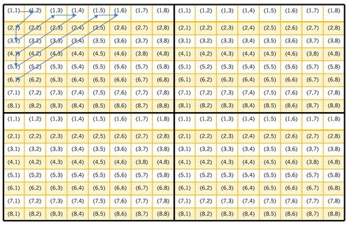
4. DCT (Discrete Cosine Transform) is applied to each block in each channel, the lowest frequency resides in the upper-left corner, and the highest frequency resides in the lower-right corner of each block.The same position in each block is called a mode. The mode table is shown below.
5. For a pre-defined quantization table (also of the size 8*8), each DCT coefficient is quantized by the corresponding the step in the quantization table, and then rounded to the nearest integer. Usually, the steps for low frequencies are small and steps for high frequencies are big, so the high frequency can be removed without much effect on human vision.
6. Encode the quantized coefficients in zig-zag order and the compression is completed.

Table 1

Double JPEG Compression

Double Compression can be regarded as a compression of a compressed image. For a compressed image, inverse quantization and inverse DCT are applied to decompress. After rounding all the values to integers, JPEG compression procedure is applied again, usually with different quantization steps. The flow of double compression of one channel is shown below.

Figure 2

Corresponding to the quantization step, another term is quality factor. The bigger the quality factor is, the better the image is, the smaller the quantization step is. In this project, for double compression, the quality factor for the first compression is named Q1 and that for the second compression is named Q2.

Method

Histograms

AC Coefficients Histogram

Usually, in the process of double compression, the two quantization steps are different, which may cause a different histogram distribution in doubly compressed images. Some people did research on the distribution of AC coefficients, and found that the distributions satisfy a Laplacian distribution, which is centered at 0, and decreases in each side. Furthermore, the distribution of the difference of nearby values also satisfy a Laplacian distribution. So this method applies this pattern to detect double compression.Since the upperleft coefficients contains the information of low frequencies, they are more sensitive to high frequencies, I choose the first 20 modes in zig-zag order, and draw the histogram of values from 2 to 10 in these modes. That is, in each mode for all blocks, I record the number of appearance of 2, 3, 4, ..., 10, so there are 9 buckets in each mode. The difference histogram calculates the difference of counts of nearby values, that mean, the first bucket stores f(2)-f(3), the second bucket stores f(3)-f(4)..., where f(x) means the number of appearance of value x in one mode. Here are two difference histogram examples, the left one is the histogram of a singly compressed image with quality factor 80, and right one is of a doubly compressed image with quality 65 and 95 separately.

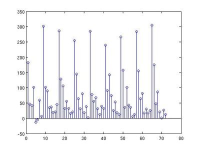
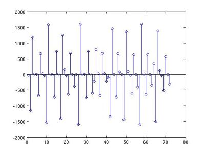
From the two histograms, we can see that the difference is obvious. By calculating the ratio of negative values in the histogram, it is easy to distinguish singly compressed image and doubly compressed image with Q1 < Q2.

First Digit Histogram

This method is based on Benford's Law. Benford's Law is also known as first digit law and is an empirical law. It was first discovered by Newcomb in 1881 and rediscovered by Benford in 1938. This law states that the probability distribution of the first digit, x (x = 1, 2, 3, ..., 9), in a set of natural numbers is logarithmic. To be specific, the distribution can be written as

math 1

Some researches were conducted on applying Benford's Law to image processing, and it was found that the distribution of the most significant digit(first digit) of the block DCT coefficients follows Benford's Law quite well and the quantized coefficients follow a Benford-like logarithmic law when the image is compressed once in JPEG format. The following two histograms verify this. They are the distributions of first digit in the first nine mode for an image compressed with quality factor 80 and an image doubly compressed with quality factor 65 and 95.

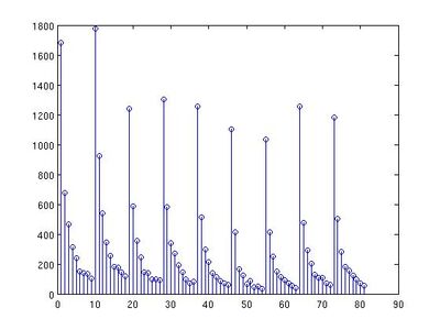
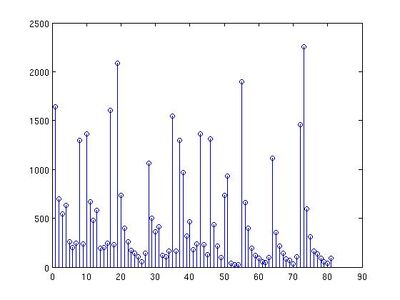
From the two histograms, we can see that the Benford's Law can be applied to detect doubly compressed image by testing the distribution of the first digits.

Factor Histogram

This method is based on a series of mathematical derivations.

c2 = [(c1q1+e)/q2] (1)

c2 – 0.5 <= c1q1/q2 < c2 + 0.5 (2)

(c2 – 0.5) q2 <= c1q1 < (c2 + 0.5) q2 (3)

D(c2, q2) = {「(c2-0,5)q2」+x|x=0,1,…,q2-1} (4)

c1q1∈D(c2, q2) (5)

F(c2, q2) = {x|mod(y,x) = 0, y∈D(c2, q2), x>0} (6)

q1∈F(c2, q2) (7)

Suppose for a doubly compressed image, the quantization steps are q1 and q2 separately, and the quantized coefficients are c1 and c2 separately. According to the procedure of double compression, we have the formula (1). The term e stands for the rounding or truncation error. In order to get a relationship for q1, q2, c1 and c2, we can ignore e here. It is obvious that formula (2) and (3) can be obtained from (1). The range of c1*q1 includes q2 consecutive integers, which can be represented as a set D, so we have formula (4), which is a set of values of c1*q1. Notice that q1 is a factor of c1*q1, so q1 is also a factor of the set D. We can represent the factor of set D using another set F, so q1 is an element in F. These are formula (6) and (7). Given a JPEG file, the quantization table can also be read from the head file. So we can easily get the set D. For each element is set D, we can obtain all the factors. By counting the number of each factor for all elements in D, we can draw a histogram, which is called factor histogram. The following two are an example of factor histograms in mode (1, 2). The left one is of a singly compressed image, and right one is of a doubly compressed image.

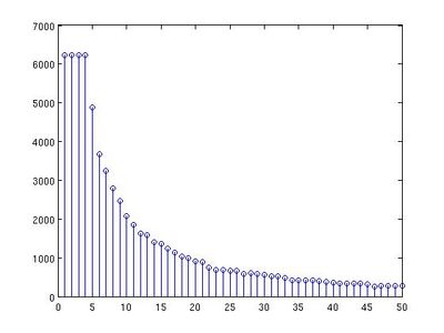
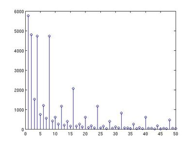
From the above two examples, we can see that the factor histogram for a singly compressed image is smooth, and that for a doubly compressed image is not smooth, so that this is a clue to detect double compression.

Markov Random Process Prediction

This method is based on the probability of transition. First define 4 directions: horizontal, vertical, main diagonal and minor diagonal. For each direction, given the coefficients matrix, we can calculate the difference matrix by the four formulas:

Fh(x, y) = F(x, y)-F(x+1, y)

Fv (x, y) = F(x, y)-F(x, y+1)

Fd(x, y) = F(x, y)-F(x+1, y+1)

Fm(x, y) = F(x+1, y)-F(x, y+1)

Based on the four difference arrays, we can calculate the transition probability. Use the horizontal array as an example. First, truncate all the elements in the array to the range of [-4, 4] in order to reduce computation. Given the current value, we can calculate the probability of next value using the formula:

math 5

δ(x = a) is one if x == a, otherwise, it is 0. For example, m = n = -4, the denominator is the total number of -4 in this array, and the numerator is the number of pairs in which the current value is -4, the next value (in the horizontal direction) is also -4. So the result of p{next = -4 | current = -4} is the transition probability of -4 to -4. Do the similar calculation for all current value and next value in the range of [-4, 4], so there would be 9*9 = 81 probabilities in one direction, and there would be 9*9*4 probabilities in all directions. These probabilities can be used as features by machine learning methods.

However, computation of this method is too large. For one image, 81 iterations are need to calculate the transition probabilities, and in order to use machine learning methods, 1000 or more images are needed to do the training, so this method is very slow and inefficient, and would be not developed further in this project.

Machine Learning

All the four above methods are very good at detection double compression with quality factor Q1 < Q2. For the opposite condtion (Q1 > Q2), the histogram patterns look very similar to singly compressed image, so other methods need to be applied. Machine learning methods could be helpful here. Specifically, I use two methods, SVM and Naive Bayes. The features for the two methods are AC coefficient histogram and first digit histogram. 400 singly compressed images and 600 doubly compressed images with Q1 > Q2 are trained. Label the singly compressed image as -1 and doubly compressed image as +1.

SVM

SVM (Support Vector Machine) is one of the best supervised learning algorithm and easy to use. In this project, I use the standard linear SVM library. For AC coefficients, the features are the counts of values from 2 to 9 in the first 20 modes, so there are 180 features for each image. For first digit histogram, there are also 180 features, but they are the counts of 1, 2, 3, ..., 9 as the first digit in each of the first 20 modes. After training the dataset, we can get a model to do the testing.

Naive Bayes

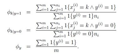
This classification method is based on the probability model p(x|y), where y is the label 1 or -1, x is the feature value. The following formulas can be applied to calculate the model and the prediction.

math 6

math 7

Final Workflow

Since different methods can be used to detect doubly compressed images with Q1<Q2 and Q1>Q2, so my detection can be divided into three parts.

1. The first part is to use simple histogram methods to detect doubly compressed image with Q1<Q2.
2. Then if the result is not true, the image could be singly compressed or doubly compressed with Q1>Q2. The second part is to use SVM or Naive Bayes to do further classification.
3. If the result is true, the image is doubly compressed, otherwise in the third part, it is classified as the singly compressed image.

Results

1. The histogram detection of doubly compressed images with quality factor Q1 < Q2 works quite well with accuracy 98%.

2. But for doubly compressed images with quality factor Q1 > Q2, their histograms cannot be differentiated from singly compressed images by simple methods, so machine learning methods are used to distinguish the two classes. The test results of my own tests for SVM and Naive Bayes are:

table 5

3. The total accuracy is around 80%.

4. For the testing images, the final results are:

table 6

Conclusion

1. It is easy to detect doubly images which is first compressed with a low quality factor and then compressed with a high quality factor. Their histograms look very different from singly compressed images in AC coefficients, factor histograms and first digit distributions.
2. In order to detect doubly images which is first compressed with a high quality factor and then compressed with a low quality factor, machine learning methods are useful. Though SVM usually performs better than other classifiers, but in this scenario, it is overfitting, because when I use the training matrix as the testing matrix, the accuracy is 100%, but the accuracy for untrained images is low. To solve the problem of overfitting, I reduced the feature size by only using the first nine modes, which results in a vector of size 9*9 = 81, but the result is still not good. In contrast, Naive Bayes has a good performance, though the TP rate is not as high as SVM, but it can correct detect some TN cases.
3. There are also many other methods to detect double compression, and furthermore, to detect the number of compression (three or fourth compression), that is a future work of this project.

Reference

1. Hany Farid, “A Survey of Image Forgery Dection”
2. A. C. Popescu, “Statistical Tools for Digital Forensics”
3. Jianquan Yang, Guopu Zhu and Jiwu Huang “Detecting Doubly Compressed JPEG Images by Factor Histogram”
4. Dongdong Fu, Yun Q. Shi, Wei Su, “A generalized Benford’s law for JPEG coefficients and its applications in image forensics”
5. Bin Li, Yun Q. Shi, JiWe Huang, “Detecting Doubly Compressed JPEG Images by Using Mode Based First Digit Features”
6. Chunhua Chen, Yun Q. Shi, Wei Su, “A Machine Learning Based Scheme for Double JPEG Compression Detection”

Appendix: Code

File:Code.zip