Back to Psych 221 Projects 2013

Background

Since digital images have become ubiquitous in the internet, the image based forgeries have become widespread as well. From the ultra slim model flashing in the cover of a fashion magazines to the manipulated images submitted to The Journal of Cell Biology[3], image based forgeries have become very common these days. The U.S Office of Research Integrity reported that there were less than 2.5% of accusations of fraud involving disputed images in 1990. The percentage rose to 26% in 2001 and by 2006, it went up to 44.1% [3]. Image Forgeries are frequently seen in forensic evidence, tabloid magazines, research journals, political campaigns, media outlets and funny hoax images sent in spam emails which leaves no doubts for the viewer as they appear to be visually acceptable without any signs of tampering. This necessitates a good method to detect these kind of forgeries. Detecting these forgeries comes under the field of Digital Camera Image Forensics. There are two main interests in Digital Camera Image Forensics. One is source identification and the second is forgery detection. Source identification deals with identifying the source camera with which an image is taken while forgery detection deals with detecting tampering in an image by assessing the underlying statistics of the image[4]. In this project, we have dealt with forgery detection.

Few examples of Forged images available on the internet

Introduction

In this class project, we have concentrated on Forgery detection by detecting changes in the underlying statistics of the image. Many digital cameras use color filter arrays in conjunction with a single sensor to record the short, medium and long wavelength information in different pixels of an image. The color information in each individual pixel is obtained by interpolating these color samples using a technique called demosaicing. This interpolation introduces specific correlations which are likely to be destroyed when the image is tampered. The goal of our project is to build a classifier in MATLAB that can take an input image and identify the parts of the image that do not exhibit the expected CFA correlations. We will use the correlation techniques described in [1] to identify parts of the image that are being tampered with.

Methods

Detecting Forgeries using CFA interpolation

We have used a method that detects tampering in images using the correlation in image pixels left by the CFA (Color Filter Array) interpolation algorithm [2]. This technique works on the assumption that although digital forgeries may leave no visual clues of having been tampered with, they may, nevertheless, alter the underlying statistics of an image. Most digital cameras, for example, capture color images using a single sensor in conjunction with an array of color filters. As a result, only one third of the samples in a color image are captured by the camera, the other two thirds being interpolated. This interpolation introduces specific correlations between the samples of a color image. When creating a digital forgery these correlations may be destroyed or altered. We have used the correlation techniques and method described in [#References |2] that quantities and detects them in any portion of an image.

CFA - Bayer Array

The Bayer arrangement of color filters on the pixel array of an image sensor

In photography, a color filter array, or color filter mosaic (CFM), is a mosaic of tiny color filters placed over the pixel sensors of an image sensor to capture color information. Color filters are needed because the typical photosensors detect light intensity with little or no wavelength specificity, and therefore cannot separate color information. The color filters filter the light by wavelength range, such that the separate filtered intensities include information about the color of light. For example, the Bayer filter (shown to the right) gives information about the intensity of light in red, green, and blue (RGB) wavelength regions. The raw image data captured by the image sensor is then converted to a full-color image (with intensities of all three primary colors represented at each pixel) by a demosaicing algorithm which is tailored for each type of color filter. A Bayer filter mosaic is a color filter array (CFA) for arranging RGB color filters on a square grid of photosensors. Its particular arrangement of color filters is used in most single-chip digital image sensors used in digital cameras, camcorders, and scanners to create a color image.

Interpolation Algorithms

A demosaicing (also de-mosaicing or demosaicing) algorithm is a digital image process used to reconstruct a full color image from the incomplete color samples output from an image sensor overlaid with a color filter array (CFA). It is also known as CFA interpolation or color reconstruction. A wide range of interpolation algorithms exist in the image processing industry and different digital camera implement different interpolation techniques. The following demosaicing techniques for the Bayer array were used by the authors of [1] to develop the detection method which is used in our project.

i) Bilinear and Bicubic
ii) Smooth Hue Transition
iii) Median Filter
iv) Gradient-Based
v) Adaptive Color Plane
vi)Threshold based variable number of Gradients

CFA interpolation based detection

The simplest demosaicing methods are kernel-based ones that act on each channel independently (e.g., bilinear or bicubic interpolation). More sophisticated algorithms interpolate edges differently from uniform areas to avoid blurring salient image features. Regardless of the specific implementation, CFA interpolation introduces specific statistical correlations between a subset of pixels in each color channel. Since the color filters in a CFA are typically arranged in a periodic pattern, these correlations are periodic.

If the specific form of the periodic correlations is known, then it would be straightforward to determine which pixels are correlated with their neighbors. On the other hand, if it is known which pixels are correlated with their neighbors, the specific form of the correlations can easily be determined. In practice, of course, neither is known. In reference paper[1], the authors employed the expectation/maximization (EM) algorithm to determine the specific forms of correlations.

Expectation/Maximization algorithm

The EM algorithm is a two-step iterative algorithm: [1]
1) in the expectation step the probability of each pixel being correlated with its neighbors is estimated; and
2) in the maximization step the specific form of the correlations among pixels is estimated.

By modeling the CFA correlations with a simple linear model, the expectation step reduces to a Bayesian estimator and the maximization step reduces to weighted least squares estimation. The E step and M step are iteratively repeated until a stable value of alpha is reached.

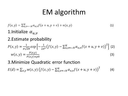
The algorithm begins with the assumption that each sample is either correlated to their neighbors in which case it satisfies equation (1) where $f(x,y)$ is the intensity matrix of the color channels, $N$ is the number of neighboring pixels included in the interpolation, $\alpha ~{u,v}~$ are the interpolation coefficients, and $n(x,y)$ is independently distributed samples drawn from Gaussian distribution with zero mean and variance $\sigma ^{2}$ ; or generated by a non correlated process.

The algorithm works as follows

1. Set initial values of N, $\alpha ~{u,v}~$ , $\sigma ^{2}$ ;
2. In the E step, probability estimate that each sample is correlated to its neighbors is calculated using equation (2) and (3)
3. In the Mstep, a new estimate for $\alpha {u,v}$ are calculated by solving equation (4) and updating the value of $\sigma ^{2}$ for that iteration.
4. Step 2 and 3 are repeated until the difference between $\alpha ~_{n}~^{u,v}$ and $\alpha ~_{n-1}~^{u,v}$ is less than $\epsilon$ which is set to a low value for a better estimate

Probability Map and Fourier Transforms

If we take the FFT of the probability map of a real part and tampered part generated using the EM algorithm, it looks as shown in the following figures. Note the peaks in the diagonal frequencies that confirms the correlation in the real image. And lack of this pattern in the tampered part. The real and tampered regions are marked in the original image using green and red squares respectively. Note that the probability map shows differences in these areas between the real and tampered regions.

[[File:plane.jpg|thumb|500px|centre|Figure 3]]

FFT of fake region - marked in red in the original image

Classifier

To detect if an image is real or fake using the EM algorithm described in the paper, we used the following two methods In both the images the image is divided into blocks of block_size*block_size Determining the difference in alpha values between adjacent blocks and declaring the image as fake if it is above a preset threshold. Determining the similarity measure of each blocks and declaring an image as fake if the similarity measure of any of the blocks are below a preset threshold

Similarity Measure based Classifier

Based on the paper [1], the similarity measure is calculated as follows

Let $p_{g}(x,y)$ be the probability map obatained from the green channel of the image and $s_{g}(x,y)$ be the green channel of the image before interpolation.
The probability map $p_{g}$ is Fourier Transformed $P_{g}(w_{x},w_{y})$ The synthetic map $s_{g}$ is Fourier Transformed $S_{g}(w_{x},w_{y})$
The Similarity Measure is then given by $M(p_{g},s_{g})=\sum \left|P_{g}(w_{x},w_{y}))\right|\left|S_{g}(w_{x},w_{y}))\right|$

We tested around 40 training image pairs and generated similarity measures to determine the threshold that can be used to classify real and fake images. As the fake images have tampering in small blocks, taking mean over all the blocks would destroy the information. So, we take the minimum similarity measure value of the blocks, normalize it with the mean value, and if it is below some threshold, it would be most likely a false image. If all three chanels are below threshold, then we classify it as a false image.

We got the following results using the training images
True positive 74.4%
True negative 60.5%
False positive 25.6%
False negative 39.5%

The threshold for each channel is red 0.47, green 0.45, blue 0.55.

Alpha difference based Classifier

Alpha difference of adjacent blocks

Since the similarity measure was not helpful in determining a single threshold, we tried other methods such as comparing the alpha values (correlation coefficients) of each block of real and fake image. The image was divided into multiple chunks with block_size set to 32x32, 64x64 and 128x128 and the alpha values obtained on real and fake images were plotted. By looking at the distribution plots, we thought that this will be a useful measure to compare the fake and real images. Even though, there are significant differences between the alpha differences from the tampered block of a fake image and the corresponding block of a real image, this method will not be helpful as we need the real image to determine which block is tampered.

Alpha difference using four neighbors

So, we decided to try if finding the alpha differences from four neighbors of a block(top, bottom, right and left blocks) and adding them helps. As you can see from the following figure, the differences between real and fake image are well pronounced. But still, this is not a good measure as windows that are not tampered also showed a larger difference in the alpha values with its neighbors.

We used the maximum difference in alpha of each image as a measure to separate the real and fake images. To determine a threshold, we plotted the histogram of red, green and blue channels of real and fake images to identify a singe value that can classify between real and fake images.

Determining Threshold

To determine the threshold that can differentiate real and fake images, the values of maximum alpha distribution were collected by testing our algorithm on different training images. The alpha_difference distribution of real and fake for the three color channel shows that many fake images have differences greater than 2 while many real images have max alpha differences less than 2.

To determine the threshold, we plotted the scatter graphs of red, green and blue channels and found that setting different thresholds for the three channels help in improving detection accuracy.

An image was classified as fake if the maximum alpha difference of all three color channels are greater than their respective threshold.

We got the following results by testing the algorithm on 40 pairs of images with two different block sizes

Window_size 128x128 - prediction accuracy 65% with the threshold for red, green and blue set to 1.8, 1.3 and 1.8 respectively
Window_size 32x32 - prediction accuracy 75% with the threshold for red, green and blue set to 1.8, 1.7 and 1.8 respectively

Compressed Images

We also tried this method on 20 image pairs compressed with the following quality factors 70, 80, 90 and 95.

The prediction accuracy was only 50% as the maximum alpha differences were in the range of 10-20 while the threshold was set to 1.8 (obtained from uncompressed training images). Since the maximum alpha differences for real and fake images were widely scattered, determining a single threshold for the compressed images seemed to be a difficult task. This is expected, as the prediction accuracy drops below 50% when the images are compressed with a quality factor below 85 due to the noise introduced by the compression [1]. Also, decreasing the quality factor destroys the correlation introduced by CFA.

Test Results

Similarity Measure

The following results were obtained by running the test images provided by Henry using the similarity measure based classifier

Threshold used for red green and blue channels are 0.47, 0.45 and 0.55 respectively

For the provided uncompressed test images we got the following results
True positive 57%,
True negative 43%.
False Positive 43%
False Negative 57%

For JPEG compressed files in the test images, the results are given below. It can be seen that this method does not perform well on JPEG compressed images.
True Positive is 33%,
True negative is 67%
False Positive is 67%
False Negative 33%

Terminologies:
True Positive - Real images identified as real
True Negative - Fake images identified as fake
False Positive - Real images identified as fake
False Negative - Fake images identified as real

Using alpha difference based classifier

Threshold used are 1.8, 1.7 and 1.8 for R, G, B channels. Block size = 32x32

Prediction accuracy = 62%

Conclusions

The similarity measure based classifier did not give a good prediction accuracy and it was difficult to set a threshold that can classify real and fake images clearly. Using separate thresholds for each of the three channels helped us in classifying images better than using single threshold for all the channels. We think that we should have used a controlled stimuli to test our algorithm and to set the threshold. We believe that it might have helped in building a good classifier based on similarity measure. Based on our findings, we believe that a single threshold cannot universally segregate between different categories (compressed, resized) of real and fake images. Using a cosine similarity measure might have helped as well.

Using the maximum alpha differences using 4 neighbors in the real and fake images seems to help classify images better.

The following are our findings
- Using the correct window size is crucial in identifying fake images. We arrived at this conclusion after experimenting with multiple window sizes. Based on our observation, setting a large window size averages the similarity measure if the tampered region is very small. Also, having a small window size brings blocking artifacts and also reduces prediction accuracy if the classifier uses methods that compare adjacent windows.
- Using information from all the three channels is helpful in building a better classifier
- As mentioned in the paper, reinterpolating a tampered image will reduce the prediction accuracy of this similarity measure based classifier approach.
- Prediction accuracy reduces if the tampered images are compressed with a low quality factor.

References

1. Farid, Hany. "Image forgery detection." Signal Processing Magazine, IEEE26.2 (2009): 16-25.

2. Popescu, Alin C., and Hany Farid. "Exposing digital forgeries in color filter array interpolated images." Signal Processing, IEEE Transactions on 53.10 (2005): 3948-3959.

3. Mahdian, Babak, and Stanislav Saic. "Detection of copy–move forgery using a method based on blur moment invariants." Forensic science international 171.2 (2007): 180-189.

4. Van Lanh, Tran, et al. "A survey on digital camera image forensic methods."Multimedia and Expo, 2007 IEEE International Conference on. IEEE, 2007.

Appendix I - Code and Data

Code

File:LiuVenkatesanYang CodeFile.zip

The zip file has a ReadMe.txt explaining the instructions to run the code.

Data

We only used the training images provided by Henryk.
We compressed the training images to generate JPG files with different quality factor to test the algorithm on compressed files

Appendix II - Work partition

All three of us collaborated equally to discuss the algorithm, method of analysis and results. We met regularly to share our ideas and to discuss the progress. We shared the task of running the tests and generating results equally.
The following is a break down of our major tasks
Yuchi Liu - Coding Expectation/Maximization algorithm, similarity measure and running respective tests
Xuan yang - Coding alpha difference of adjacent neighbors, code to compress images with different quality factors and running respective tests
Preethi Venkatesan - Coding alpha difference between 4 neighbors, automated code to accept multiple images and determining threshold that maximized detection accuracy and running respective tests

LiuVenkatesanYang

Contents

Background

Introduction

Methods