Murthy
Introduction
The study of human eye movements and vision is an active research field. Over the past 35 years, researchers have focused on a few particular topics of interest, namely smooth pursuit, saccades, and the interactions of these movements with vision. The fundamental question of “how does the motion of the image on the retina affect vision?” has been a continuous area of focus.[1]
The knowledge of how eye movements impact vision has a wide variety of beneficial implications, from augmenting understanding of human behavior to assisting in the development of therapeutics. Eye movement studies have been used since the mid nineteenth century to understand human disease [2], and applications of eye movement research have the potential to alleviate vision disorders (such as the Stanford Artificial Retina Project, which can utilize such research to inform the prosthesis design).[3]
The study of eye movements and their impact on visual acuity can be challenging to conduct in vivo. Noise can be introduced from uncontrollable oculomotor muscle contractions, and it is challenging with human participants to perform repeatable eye movements and obtain an objective measure of their effect on vision. The ISETBio toolbox provides comprehensive functionality to enable the study of human visual acuity in a controlled simulation environment.[4]
The purpose of this project is to modify the eye movement patterns and cone properties of an ISETBio visual model, and observe trends related to the effects of these parameters on the visual acuity of the model. For this project, the Modulation Transfer Function (MTF) is used as an evaluation of visual acuity. The MTF is a curve depicting contrast reduction vs. spatial frequency, and it is a widely accepted research and industry standard method of comparing the performance of two visual systems.[5]
Background
In this project, both photoreceptor properties and eye movements may have an effect on visual acuity.
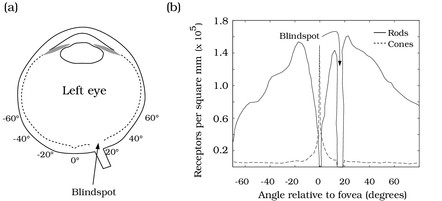
With respect to photoreceptor properties, it is known that both cone density and cone type vary as one moves across the retina. As described in Foundations of Vision, the very center of the fovea (defined as 0 degrees of eccentricity) has a photoreceptor distribution consisting entirely of cones. Specifically, there are only L and M cones at this location on the retina [6]. As one moves more peripherally, the concentration of cones decreases and the distribution of cone types changes. L, M, and S cones are all present, and the size of the cone apertures increases as one moves peripherally from the center of the fovea [6]. Different cone types (L, M, S) are sensitive to different wavelengths, and therefore have different individual point- and line-spread functions. It is known from lecture that S cones have a larger point-spread function than M and L cones. Both cone aperture size and cone type could be expected to have an impact on visual acuity in different regions of the retina.
With respect to eye movements, there are three distinct types of eye movements that are commonly studied: fixational, nystagmus, and drift. It is known that our eyes constantly move while fixating on an image. One theory surrounding fixational eye movements is that they are necessary to maintain good vision because photoreceptors and retinal ganglion cells can fatigue under constant stimulus. The fixational movement provides a constantly, slightly changing stimulus, eliminating the fatigue. This fatigue theory acknowledges that this benefit likely comes at the cost of decreased visual acuity [7]. This project will try to investigate this fatigue theory.
Nystagmus is defined as repetitive, oscillatory “to-and-fro” eye movements that are rapid and involuntary. It is known that the movement associated with nystagmus is associated with a shift of the retinal image and a decrease in visual acuity [8]. It is interesting to therefore further investigate how the orientation and amplitude of nystagmus movements impacts visual acuity. Drift movements, in the context of this project, are defined as much slower movements than nystagmus. These movements are intended to mimic everyday, normal eye movements to see how they affect visual acuity as compared to the other eye movements.
Methods
MTF Computational Pipeline
ISO12233 provides a method for computing the MTF in a fast, standard manner. The MTF is, by definition, the magnitude of the Fourier Transform of the Linespread Function of the optical system. In turn, the Linespread Function is the derivative of the system’s response to an edge [9]. Using ISETBio and its ISO12233 function, the MTF can be generated by presenting a slanted edge to the visual model and performing the aforementioned calculations to get from the edge response to the MTF curve.
In this regard, all MTFs for this project were generated via the computational pipeline depicted in Figure 1. First, the “slanted edge” scene is generated. A macular pigment is applied to obtain the optical image of the scene. Second, a cone mosaic is created to produce the retina model. This process is described in more detail below. Third, the eye movement sequence is generated. This process is also described in more detail below. Fourth, the optical image is presented to the cone mosaic. The photon absorptions of each cone in the mosaic are computed for each time step (in this project, 5 milliseconds). Every time step, the presented image is shifted in accordance with the single eye movement for that time step. Finally, the mean absorptions for the cone mosaic are used to generate the MTF via the ISO12233 function. This process is repeated for the desired number of trials, producing one MTF per trial.

Generating Cone Mosaics
In order to execute the process depicted above, it was first necessary to generate the cone mosaics that would be used. For this project, it was desired to model two portions of the retina- the center of the fovea, and slightly to the periphery. For each model, a rectangular cone mosaic was generated using the “coneMosaic” method in ISETBio.
First the “center” model was created. This cone mosaic is meant to represent the photoreceptors at the center of the fovea. Using the knowledge from Foundations of Vision that the S cones are absent at the center of the fovea [6], this model was created by specifying an even distribution of L and M cones, with no S cones and no blank spaces. The “coneMosaic” method in ISETBio defaults to generating cones with an aperture that is representative of the center of the fovea, so no special parameters needed to be set with respect to aperture. In this model, the aperture size was 1.4 micron. The “center” cone mosaic is depicted in Figure 3 below.
Second, the “periphery” model was created. This cone mosaic is intended to represent the photoreceptors at a few degrees eccentricity relative to the center of the fovea. Initially, I considered making a mosaic that included blank spaces, which would represent rods. However, when attempting to run the ISO12233 routine using a model with blank cones, the resultant MTFs either failed to compute or had erroneous shapes, indicating computational difficulty.
To address this issue while still attempting to generate a relatively accurate retinal model, the periphery model was chosen to represent 2 degrees of eccentricity. This decision was based on Figure 3.1 from Foundations of Vision (linked) [6], which depicts the density of rods and cones as one moves across the retina. It is clear to see that while cone density falls off rapidly as one moves peripherally from the fovea, there is still a high concentration of cones at 2 degrees of eccentricity. To determine the aperture size for these cones, the ISETBio function “coneSizeReadData” was used. This function uses data from Curcio et. al. (Figure 6), in Figure 2 below, to estimate cone aperture size from cone density data [10]. Using this method, the cone aperture size for the periphery model was 3.89 micron. The relative density of L, M, and S cones is 60%, 30%, and 10% respectively, based off a claim in Foundations of Vision [6]. This mosaic is also depicted in Figure 3 below.


Generating Eye Movement Sequences
For this project, it was desired to create a wide variety of relatively realistic eye movements. In addition to specifying a blank set of eye movements to provide a stationary baseline for later comparison, the three aforementioned eye movement types were modeled: fixational, nystagmus, and drift. All sequences were coded into the model by setting the “coneMosaic.emPositions”.
First, the fixational eye movements were generated. These were made by using the ISETBio built-in functionality, which defaults to the creation of random, small amplitude microsaccades.
Second, the nystagmus eye movements were added. These sequences could not be generated using a built-in ISETBio function, so they were custom programmed. Nystagmus is characterized by rapid, oscillatory eye movements, so these sequences consist of rapid flicks of the eyes back and forth. With these movements, it was desirable to investigate the effects of orientation and amplitude on the resultant visual acuity. Therefore, four separate Nystagmus sequences were created – horizontal, vertical, parallel, and perpendicular.
For the horizontal and vertical sequences, one specifies an amplitude in number of cones on the cone mosaic. The eye positions flick between the positive and negative values of that amplitude with each time step. To attempt to make the movements slightly more realistic, a “jitter” parameter was also added that created a small amount of perpendicular movement. For example, one horizontal sequence could have an amplitude of 8 cones to the left and right, but then “jitter” up and down by 1 or 2 cones. This is meant to model oculomotor contractions, which will not necessarily be perfectly along one axis.
For the parallel and perpendicular sequences, the amplitude is fixed to be ~5 cones. The parallel path is designed such that its slope matches the slope of the slanted edge that is being presented to the visual model, and the perpendicular path is perpendicular to the slanted edge scene.
The fixational and nystagmus movement sequences are depicted in Figure 4 below.

Finally, the drift sequence was added. For this sequence, it is only horizontal, and there is no jitter involved. One can specify an amplitude in cones of the mosaic, and the eye will drift to the positive and negative of that amplitude, but will only do this once over the entire course of the movement sequence. This is a much slower movement in relation to the nystagmus movements. The difference between the drift and nystagmus sequence can be seen in Figure 5 below.


Automated Script
To allow investigation of the effects of these input parameters on the output MTF, a MATLAB script was developed to automate the MTF generation process. This script is attached in Appendix I, and can be used by current and future students to both validate the results presented here and to continue similar investigations in future projects. The script allows a user to specify which model type they’d like to use (and define degrees of eccentricity for the periphery model), select one type of eye movement pattern (and set defining characteristics such as amplitude), specify the number of eye movements and number of trials, and specify whether photon noise is present. Once those parameters have been defined, the script will run the desired number of trials, store all MTF info from the ISO12233 routine, and plot all the MTFs in one figure. It will also keep track of some characteristic statistics, as will be discussed further in the Results section.
Results
Noise
Upon beginning to modify parameters and generate MTFs, it quickly became clear that the MTF curves being generated were not consistent from one run to the next. Three sources of noise were identified as contributing factors. (1) The cone mosaic pattern was randomly generated. Although the ratio of cone types was consistent, their particular locations were not. (2) Photon noise was present in the model. This is a physically accurate representation that is built into the ISETBio cone absorptions. (3) Certain eye movement patterns had variability. Fixational eye movements were randomized, and the “jitter” components of nystagmus were random.
To attempt to eliminate this noise and look first at the cleanest possible trends between input parameters and effect on MTF, a third cone mosaic model was generated, referred to as “control”. This mosaic consists entirely of L cones, has the same standard foveal cone aperture of 1.4 micron, and has photon noise disabled.
Not all of the noise could be eliminated from the control model, as some eye movements still had randomness. Furthermore, it would be necessary to add noise back in when assessing the center and periphery models. To account for this variation in MTF curves, the MTF50 metric was identified as a proxy for visual acuity. This metric represents where contrast reaches half of its peak, and it is a standard way of comparing optical systems. Since the MTF50 was relatively consistent across many trials with variable MTFs, the mean MTF50 provides a good indication of the visual acuity of the system, and the standard deviation of the MTF50 can help quantify the variability across trials. These statistics were built into the automated test script previously mentioned.
Control Model Trends
The repeatable MTF resulting from the control model and no eye movements is in Figure 6 below. This is the benchmark to compare against for visual acuity. The MTF50 value for this scenario was 10.95 cycles/degree.

When running the control model with 50 fixational eye movements per trial, for 100 trials, the MTF output is in Figure 7 below. It is clear that the MTFs vary considerably in the higher spatial frequency portions of the plot. However, the MTF50 value remained fairly consistent, which can be seen in Figure 7 as well. The mean MTF50 was 7.51 cyc/deg for this scenario, and the standard deviation was 0.7674 cyc/deg. This indicates visual acuity markedly decreased with fixational eye movements.

This finding agrees with Martinez-Conde et. al. and their fatigue theory [7]. To investigate whether fatigue could have occurred, I briefly looked at the cone photocurrent values on the first and last time step for the scenario without eye movements. The mean photocurrent absorptions were approximately the same for each (both were ~45), which indicates photoreceptor fatigue was not built into the ISETBio model.
When investigating the Nystagmus patterns, again with 50 eye movements and 100 trials, it was found that the mean absorption image was greatly affected by the orientation of the eye movements in relation to the slanted edge. The more perpendicular the movement was to the edge, the greater the blur effect in the absorption image. This is demonstrated in Figure 8 below.

Logically, this blur effect had an effect on the resultant MTFs. The photon noise-less MTFs for the two extremes, the parallel and perpendicular nystagmus movements, are in Figure 9. It is clear to see that the parallel MTF closely resembles the benchmark no-movement MTF in Figure 6. However, the perpendicular MTF suffers a rapid decline in contrast, and has an MTF50 value of approximately half that of the parallel. This indicates that one’s visual acuity with respect to an edge in an image depend on the orientation of one’s eye movements in relation to that edge.

Finally, drift movements were considered. All of the results for the MTF50 means and standard deviations are in the table in the Final Results Table section.
Together with the results of horizontal and vertical nystagmus movements with differing amplitudes, the drift movements demonstrate two trends. First, the amplitude of the movements affects visual acuity, with higher amplitude movements causing a decrease in acuity. Second, the horizontal drift MTF50s for each amplitude were higher than the horizontal nystagmus MTF50s for the same amplitudes, indicating that faster eye movements lead to a further decrease in visual acuity.
Center and Periphery Model Trends
The investigations conducted with the control model were all repeated for the center and periphery models, with the presence of photon noise, 50 eye movements per trial, and 100 trials each. In total, this corresponds to over 65 MTF plots being generated. The results can be much more cleanly compared in table format, which is found in the Final Results Table section.
In the center model, all trends observed in the control model held consistent. This can be seen by observing the table. The standard deviations of the MTF50s increased, which is natural with the increase in noise in the model.
With the periphery model, the trends still held consistent as well. However, it is worth noting a few points about the periphery model. The standard deviations of the MTF50s were significantly higher in this model, in part due to the fact that the ISO12233 routine seemed to struggle with some of the computations. Figure 10 below depicts example MTFs for the center model and periphery model respectively. It is clear to see that the periphery model MTFs are at times erroneously high. Due to this, care was taken to exclude erroneously high MTF50 values, by constraining all MTF50 values used in the statistics to be less than 15 cycles/degree.

On aggregate, the visual acuity was worse with the periphery model than with the center model. This makes sense, as the cone apertures were larger and would lead to increased blur. Furthermore, the spread functions of S cones is larger than that of L and M cones, which could have been a contributing factor too.
Final Results Table
For each eye model and movement sequence in the table below, 50 eye movements were used, and 100 trials were conducted. While the trends in the table should be replicable using the attached script in the Appendix, the values are subject to change due to the noise factors previously discussed.

Conclusions
Key Findings
To summarize:
Fixational eye movements were found to reduce visual acuity as compared to a stationary eye baseline, which is in line with part of the fatigue theory. However, the full fatigue theory could not be validated because fatigue is not currently built into the cone absorptions in ISETBio.
The orientation of nystagmus movements was found to be highly correlated with visual acuity. The closer the movements are to matching the slanted edge orientation, the smaller the distortion of the scene over the mean cone absorptions, and the higher the visual acuity. Lower amplitude eye movements were associated with higher visual acuity. Slower eye movements were associated with higher visual acuity.
These trends all held for both the center and periphery models. Overall, the periphery model was found to have diminished visual acuity as compared to the center model. It also had much higher MTF50 standard deviations, due to computational challenges with the ISO12233 routine.
Limitations and Future Work
One major limitation of this investigation was the fact that the cone mosaic pattern was generated randomly for each individual movement type. For example, the center model mosaic for the fixational eye movements was different than the one for drift eye movements. This is not ideal for a controlled experiment, as one person's eye would only have one mosaic. The results presented here therefore implicitly assume that the relative distribution of cone types matters more than the specific location of those cones in the mosaic.
Another limitation was the computational challenge that occurred with the ISO12233 routine. A future project might investigate if there is a way to improve that script, potentially enabling this investigation with a retinal model that has blank spaces to represent rods.
As mentioned, the fatigue theory could not be validated because fatigue was not currently built into the ISETBio cone absorptions. A future project could add this functionality into ISETBio, either at the photoreceptor level or by adding retinal ganglion responses.
Finally, the script used to do all of this analysis is provided in the Appendix, and it has been designed to allow a user to quickly generate desired MTFs. Future work could clean up this script and add functionality, such as even more types of eye movement sequences.
References
[1] – Kowler, Eileen. “Eye movements: The past 25 years.” Vision Research. 2011. Link
[2] – Shaikh, Aasef G. and Zee, David S. “Eye Movement Research in the Twenty-First Century—a Window to the Brain, Mind, and More.” The Cerebullum. 2018. Link
[3] – The Stanford Artificial Retina Project. 2019. Link
[4]- Wandell, Brian et al. ISETBio. Github Link
[5]- Zheng et. al. “Analysis of the optical quality by determining the modulation transfer function for anterior corneal surface in myopes.” International Journal of Opthalmology. 2012. Link
[6] – Wandell, Brian A. Foundations of Vision. Link
[7]- Martinez-Conde, Susana et. al. “The Role of Fixational Eye Movements in Visual Perception.” Nature Reviews: Neuroscience. 2004. Link
[8]- Yao, Jun-Ping et al. “A new measure of nystagmus acuity.” International Journal of Opthalmology. 2014. Link
[9]- Estribeau, M. and Magnan, P. “Fast MTF measurement of CMOS imagers using ISO 12233 slanted-edge methodology.” Integrated Sensors Laboratory. Link
[10]- Curcio et al. “Human Photoreceptor Topography.” The Journal of Comparative Neurology. 1990. Link
Appendix
Visual Acuity and Eye Movements Script, Github
Acknowledgements
I would like to thank Professor Brian Wandell for his mentorship throughout the completion of this project. I’d also like to thank Prof. Joyce Farrell and Zheng Lyu for their continuous support and quality instruction throughout the course.