Psychophysical assessments of Portilla and Simoncelli's texture synthesis algorithm
by Andrés Gómez Emilsson
Introduction
When we look at a textured surface we are able to perceive many patterns and features. From a first-person perspective it is difficult to describe the exact properties of the textures we perceive. Yet we can readily access a wide variety of qualities from experience alone. Speculatively, people may someday develop a refined enough vocabulary for visual patterns to be able to talk about the subtle differences between texturized surfaces. Currently, that task is beyond us.
If everyday language is currently inadequate for the task, what can we do? Thanks to persistent interest in texture synthesis, graphics research in the last 20 years or so has developed a language to describe textures meaningfully. This language is based on statistics, and it provides a way to point out relevant and perceivable features of textures.
To what extent the current statistical properties we are able to measure and grasp mathematically truly describe the textures that we perceive subjectively is an open question. On the one hand, we don't know to what extent we really do perceive the properties modeled by the field. And on the other, we don't know if there are other features we do perceive that current statistical approaches are entirely blind to.
This project is an attempt to contribute to that conversation: By testing the ability of people to differentiate between textures with ground-truth statistical features known a priori (by construction, using texture synthesis algorithms), we aim to bridge the gap between the mathematical statistical vocabulary of visual patterns, and what stands out in our subjective experience.
Background
Portilla & Simoncelli's Algorithm
Portilla & Simoncelli developed a texture synthesis algorithm inspired by neurobiology in 1999. The algorithm analyzes an input texture and extracts a set of statistical features that describe the texture. This is called the texture analysis step. Then, in the texture synthesis step, a Gaussian noise image (of any size, even bigger than the input texture image) is iteratively made to conform to the statistical features extracted from the original image in the texture analysis step.
This algorithm is a refinement of an earlier version that uses pyramid decomposition of images. The core statistical feature captured by the texture analysis step of pyramid decomposition is the partition of the input texture into "texture pyramids" that represent oriented spatial frequency bands of the original image. This Pyramid-based texture analysis and synthesis algorithm was proposed by David Heeger and James R. Bergen. It is worth noting that this algorithm was inspired by neurobiology. Namely, empirically discovered oriented Gabor-like receptive fields of neurons in the primary visual cortex are capable of decoding the same information from an image as the pyramid decomposition.
Portilla and Simoncelli's algorithm incorporates further statistical features:
- Marginals
- A set of first order statistics. This includes the mean luminance, variance, kurtosis and skew.
- Subband Correlation (also called "Raw Auto")
- The local autocorrelation of the low-pass pyramid decomposition levels.
- Magnitude Correlation
- The autocorrelation between adjacent filter magnitudes. This includes adjacent filters in space, orientation and scale.
- Phase
- Cross-scale phase statistics. For each subband, the local relative phase between coefficients within it is computed and compared to the that of the immediately larger subband.

As described in Balas (2006):
"The Portilla–Simoncelli model utilizes four large sets of parameters to generate novel texture images from a specified target. In all cases, a random-noise image is altered such that its distributions of these parameters match those obtained from the target image. The first of these parameter sets is a series of first-order constraints (marginals) on the pixel intensity distribution derived from the target texture. The mean luminance, variance, kurtosis and skew of the target are imposed on the new image, as well as the range of the pixel values. The skew and kurtosis of a low-resolution version of the image is also included in this set. Second, the local autocorrelation of the target image's low-pass counterparts in the pyramid decomposition is measured (coeff. corr), and matched in the new image. Third, the measured correlation between neighboring filter magnitudes is measured (mag. corr). This set of statistics includes neighbors in space, orientation, and scale. Finally, cross-scale phase statistics are matched between the old and new images (phase). This is a measure of the dominant local relative phase between coefficients within a sub-band, and their neighbors in the immediately larger scale. Portilla and Simoncelli report on the utility of each of these parameter subsets in their description of the model, but offer no clear perceptual evidence beyond the visual inspection of a few example images. The current study aims to carry out a true psychophysical assessment, in the hopes that doing so will more clearly demonstrate which statistics are perceptually important for representing natural textures."
Texture Synthesis Examples
In order to grasp the concepts handled in this project it is worth becoming familiar with the ways in which the texture synthesis parameters (statistical features enforced) influence the look and feel of natural images. The following images were synthesized for this project using the Matlab code available here.
The specific source images are found here, and the adapted Matlab code for this new synthesis is found here.
This first series of images is built around a "natural scene" image of interlacing branches. Which one of the synthesized images looks the most different from the original one?
-
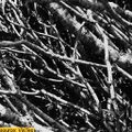 Original
 -
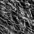 Marginals
 -
 Subband Correlation (also called "Raw Auto")
 -
 Magnitude Correlation
 -
 Local Phase (also "Phase")
 -
 Full Set


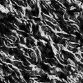
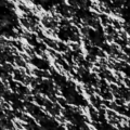
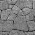
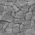
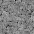
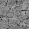
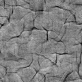
And in this second series we have a source image coming from a picture of a stone wall. Again, which is the most different synthesized picture?
-
 Original
 -
 Marginals
 -
 Subband Correlation (also called "Raw Auto")
 -
 Magnitude Correlation
 -
 Local Phase (also "Phase")
 -
 Full Set


As you may have gathered, the texture synthesis algorithm is able to capture impressive qualitative aspects of the original image. Something that it does not seem to reproduce, though, is the semantic component of the source image. While the look and feel of the synthesized "branches" and "stone walls" share a lot of qualities with branches and stone walls... you don't actually see branches and stone walls in there. An intriguing research question that naturally arises from this series of images is: To what extent do we perceive images in terms of "stuff" and to what extent we perceive them in terms of "objects." The synthesized images are clearly more "stuff" than "objects." At first you may not see a lot of differences, but as soon as you notice the object in the original pictures, all of the synthetic ones suddenly seem artificial.
Experimental Methods
In order to determine the relative importance of each of the enforced statistical features in achieving perceptual similarity, Benjamin Balas ran two experiments for his 2006 paper "Texture synthesis and perception: Using computational models to study texture representations in the human visual system". For this project, only one experiment is reproduced. Balas' goal was to understand how each of the statistical features that the Portilla and Simoncelli's algorithm enforces contributes to the overall "confusability" of the images. He ran an experiment in which he created synthesized pictures that lacked one statistical constraint (experiment 1) and another in which the synthesized images only enforced one statistical feature (experiment 2). This is with the caveat that for experiment 2 the "marginals" constraint was enforced in all of the synthesized pictures because not doing so makes the differences very noticeable.
For my replication only experiment 1 is presented. You can try it out online here yourself. Note: You can find how many correct trials you got by returning to the initial page after you are done and looking for the variable "total_correct" (which includes the check trials, as will be explained below).
Mechanical Turk
My replication used the online service Amazon Mechanical Turk to recruit participants. This service allows you to employ a large number of people to perform tasks such as surveys, proof reading, and psychology experiments.
Note: Running the experiment in Mechanical Turk was done as a replication project for the class Psych 254 taught by Michael Frank this quarter. The analysis found below, which seeks to explain the results using retinal images, was done for Psych 221 exclusively. As a whole, the project overlaps with the other class, but give then breadth and scope (and ambitiousness of it for a single project member) it fulfills the requirements for both classes.
Trials and Participants
- Original study
- 8 Participants, 2160 trials per participant
- Replication
- 60 Participants, 60 trials (plus 6 "check trials" and 4 "example trials")
In the replication participants were paid 65 cents. On average, participants took 7 minutes and 7 seconds to complete the task from start to finish, including instructions and optional comments (I originally estimated they would take at most 5 minutes).
Presentation Time
Both experiments use a standard 250 millisecond presentation time for all of the stimuli. The original experiment used Matlab Psychophysics Toolbox (Brainard, 1997; Pelli, 1997) to control this and other variables of the experiment. The presentation time in the replication was controlled using the javascript function setTimeout.
Stimuli
Below is an example of the actual stimuli used. The images were cropped just as in Balas (2006).
-
 Original
 -
 Marginals
 -
 Subband Correlation (also called "Raw Auto")
 -
 Magnitude Correlation
 -
 Local Phase (also "Phase")
 -
 Full Set


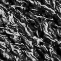
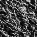
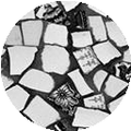
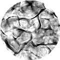
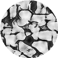
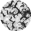
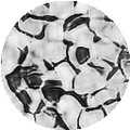
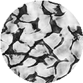
Balas' study used three kinds of images: "structured", "pseudoperiodic" and "asymmetric." The replication focused on the "Structured" images only. A total of 6 different "structured" image sources (from natural scenes corresponding to branches, ice bricks in a black background, black ovals in a white background, oval stones arranged to cover a wall, mosaic of porcelain and blocks of rock making up a wall) were used. The same textures were used for the original study. The only difference in the stimuli is that I resynthesized all of the synthetic textures.
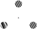
The experiment used an "odd one out" (or "oddball") paradigm to determine whether participants were able to distinguish between original and synthetic images. In brief, for a given condition (say, "full set", where all of the statistical features are enforced) three images were presented (either one original image and two synthetic, or vice versa).
The images were presented at the corners of an equilateral triangle. Each image was displayed 3.5 degrees away from the fixation point. Each image has a diameter of 2 degrees of vision with a resolution of 64 pixels/degree.
-
 Calibration
 -
 Example trial
 -
 Check trial
 -
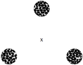 Real trial


For the replication I used 60 trials in total, using 12 trials for each condition. Of the 12 trials for each condition, each source image appeared twice, and within that pair the synthesized and original textures were the minority exactly once. The order of the trials was chosen at random for each participant.
Calibration
To roughly approximate the degrees of vision prescribed in the original experiment, we can take advantage of the known approximation that the width of one's thumb at arm's length is around two degrees of vision. The 2-degree wide blue circle is presented at the right corner of the triangle. Participants are then requested to extend their right arm in front of them with their thumb sticking up. They are asked to place the thumbnail between their right eye and the blue circle (by closing their left eye). Then the indication is to adjust the distance between their head and the computer screen until the thumb is covering the blue circle as precisely as possible.
This method is probably not highly precise. Nonetheless it roughly standardizes the degrees of vision at which the stimuli is presented.
Example Trials
Four "example trials" were presented at the very beginning, right after the calibration step. These example trials are meant to be easy and provide a few practice rounds (with known answers) for the participants to get acquainted with the task. Also, the images in the example trials are displayed for 2 seconds (except the last one, which is shown for 250 milliseconds) to slowly acclimatize participants to the difficulty of the real trials.
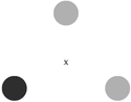
Check Trials
The check trials are easy trials interleaved with the real trials. They were introduced in the replication to make sure that participants understood the instructions and were paying attention. These trials used solid grey-scale circles with different luminance levels, as shown in the picture above.
Experimental Results
Here we make a side-by-side comparison between the results obtained by Balas and those obtained in the Mechanical Turk replication:


(Error bars in left plot represent SEM; Error bars in the right plot represent 95% CI computed using a beta prior on the probability of success for a binomial distribution - found in R's binom library).
What is worth noting here is that there is a qualitative replication. Removing the Marginals produces the largest increase in accuracy, followed by the effect of removing the Magnitude Correlation statistic. Using a proportion test we verified that these differences are highly statistically significant (p < 0.001). The same is true if any other statistical test to determine the deviation of an empirical accuracy in binary tasks with a null probability - in this case 1/3 - is used.
The last column of the replication bar plot represents the accuracy for the check trials. As you can see, the accuracy for this trials is significantly higher than that for any other condition. This suggests that participants understood the instructions and made a genuine attempt at performing the task.
However, the replication does not match the original study in a few very important ways: First, the accuracy values themselves are very different. It appears that Mechanical Turk users perform much worse than the subjects in the original study. This effect is so pronounced that we even see accuracy values not significantly different from chance levels for the Raw Auto, Phase and Full Set conditions.
This pronounced difference in performance could be accounted for in one of several ways. We will come back to this point in the discussion section. In the meantime, it suffices to point out that the Mechanical Turk experiment cannot guarantee that participants are (1) really trying their best, and (2) that lighting, monitor brightness and distance from the monitor are being controlled. In addition, the original study used only 8 subjects (who could be particularly competent) and each performed over 2000 trials. Thus, learning effects cannot be ruled out. That said, in the span of 66 trials (including the check trials), the participants in the recent study did not show any appreciable learning (the probability of an accurate response does not change as a function of the trial number).

Images in the Retina
A legitimate question we can raise about the empirical performance on this task is "what are the relevant factors that aid participants in discriminating between textures?"
Even though the texture synthesis algorithm is designed in such a way as to control for specific statistical features, it may still be the case that the reason why participants are able to identify the odd one out on a given trial is not that a picture is missing one (or has an additional) statistical feature the algorithm controls for. Instead, maybe there is a different characteristic that can be used to differentiate between the synthetic and the original textures.
In other words, maybe there is a way in which synthetic and original images are different that is not accounted for by the statistical features that Portilla and Simocelli's algorithm controls for. In such a case, we have to think about the possible sources of information that could provide hints that participants would take advantage of to identify the oddball on a given trial.
In addition, it is also the case that controlling differences in the information contained in a displayed image is not necessarily the same as controlling differences in the information available to the eye.
ISETBIO
We now turn to the biological module of the Image Systems Engineering Toolbox (ISET) to address the question raised above. Specifically, we investigate whether there is any readily available piece of information that isn't one of the enforced statistics in the textures presented during each of the real trials that could explain the performance. In other words, this is to determine whether the higher-than-chance performance on the marginals and magnitude correlation condition can be explained without invoking the ability to extract the statistical features that ultimately make the synthesized textures different from one another.
The full code is available here. Navigate to the file "Andres_clean_analysis.m" to see the code that was executed to obtain the results presented here.
Display and Optics
The Display used is 'OLDE-Sony' and the scene is created with the method "sceneFromFile."
Sensor
The sensor is set to 'human.' An important detail is that setting the sensor to behave like the human retina with a certain amount of eccentricity requires some care. Specifically, sensor.pixel.width, sensor.pixel.height, sensor.pixel.pdWidth (photodetector width) and sensor.pixel.pdHeight (photodetector height) had to be modified to account for a different number of cones per square millimeter.
Let eyeimage(texture) be an Array of electron values obtained that correspond to what the retina receives when presented with a texture image. In order to obtain eyeimage(texture) we interpolated two photon density maps that were produced with the cone density of 3.5 and 5.5 degrees of vision (roughly 20,000cone/mm^2 and 15,000cone/mm^2 respectively). Thus, the specific sensor used is intended to have a gradient of cone densities to simulate the difference between the part of the stimuli closest to the fovea and that furthest away.

The specific interpolation method is tricky to explain, but it will suffice to say that the results are indistinguishable no matter which interpolation method I employed. However, to point in the right direction, I created two sensors and then interpolated the resulting photon maps by weighting each of them accordingly as a function of the number of degrees away from the center. Ideally we would want to produce a sensor that has the actual empirical distribution of cones encoded, but this was not possible for this project, and an approximation was used.
Resulting Images
We obtain retinal images that look like these:


The leftmost image is an "original image" (i.e. the input image for the texture analysis step). The other two images are synthesized textures that have the Marginal constraint removed. As you can see, there is a gradient of luminosity from bottom to top.
Simulations
Now we will use properties of the retinal images to identify the odd one out in a set of three. The simple heuristic used here goes as follows: For a given first order statistic of the images (such as mean photon count, standard deviation, kurtosis, etc. for cones in the retina), the two images with the smallest difference are clumped together and the third image is classified as the odd one out. Here the "statistic" is not the same as the statistical feature removed. The statistical feature removed simply determines the condition of the experiment (full set, marginal, etc.), whereas here when I refer to the "statistic" I mean it in the sense of first order properties of the distribution of photons that reach the receptors in the retina.

For a given statistic (in this case mean number of photons in the retinal image) this heuristic identifies the pair of images whose selected statistic has the smallest difference. In the image above, this is represented by the short yellow line (where the x-axis represents the values for the chosen statistic, i.e. the mean). The remaining image is labeled as the "oddball." The problem with using this heuristic is that it is unreasonable to expect that the visual system is capable of estimating these statistics with extreme precision. For that reason, a more realistic version of this heuristic is used. Specifically, there is some Gaussian noise in the estimated statistic:

Thus we can look at the accuracy for various statistical features removed (marginals, magnitude correlation, etc.) as a function of the amount of noise (namely, the standard deviation of the Gaussian noise).
For each of the possible valid triads (where there is either one synthetic and two different originals or vice versa, and the set of three images are all products of the same original image kind (branches, mosaics, etc.)), we perform the above heuristic 30 times for each level of noise chosen. We count the decision as a correct inference every time the odd one matches the ground truth (the picture that belongs to a different condition). Likewise, each of the misclassifications are counted as misses.
In other words, what this simulation achieves is the following: Assuming that a person's visual system is using the information already available at the retina to identify the odd one out, we postulate a noisy biological estimator of first order statistics for those images, such as the mean number of photons. We are therefore computing the expected proportion of correct inferences in the experiment by assuming that there is only one noisy statistical feature available for classification. We will only present the results of using the mean number of photons in the following section. However, the results are very similar when we use instead the Standard Deviation (and less so for Kurtosis and Skewness).
Results
Classification performance of the heuristic
We see that exclusively using a noisy one-feature classifier that employs a heuristic (identifying as the odd one out the image that does not have the closest difference to another image among the three differences in the mean number of photons) produces very similar results to the empirically observed results.
In other words, it is possible to explain the observed performance in the replication by merely focusing on the mean number of photons that reach the cones in the retina without having to invoke the original higher order statistical features that were the focus of the experiment.
This is puzzling because the algorithm was designed to control for the luminance of the image (except the "Marginals" condition, which does not enforce this average in principle, but typically creates images with similar RGB values as the original image). These results are extremely robust: The (nearly) exact same pattern arises whether the we use 4, 3, 2 or 1 cone receptor types. This suggests that the statistical differences are found in the luminance, and do not require any cone receptor specificity.
Here is the accuracy bar plot when we have no noise:

And the classification accuracy when there is a Gaussian noise with a standard deviation of 4,000 photons.

As you may realize, there is a very significant similarity between the image above and the accuracy proportions on the replication. Finally, here is the decay of accuracy for the two most detectable features: Marginals and Magnitude Correlation. As in the empirical measures of accuracy, these two features are the most accurate. Also, the order of accuracy is also correct.

Note: The error bars are so small (given the sampling procedure) that they do not appear on the bar plots (which is why I left them out).
Classification on the raw unprocessed stimuli
What about performing the same simulations but using instead the RGB values of the unprocessed images? In other words, instead of identifying the odd one out using statistics available at the level of photons reaching the retina, what would happen if we simply use the RGB values of the stimuli?
In brief, it turns out that this sort of classification heuristic is completely ineffective at that level, delivering results always consistent with chance-level performance. This is regardless of the noise level: At every noise level, including zero noise, the classification accuracy is indistinguishable from chance.

This isn't really surprising once you consider that the first order statistics of the source textures is enforced in the synthesized texture.
The take home message is that there is already enough information to explain the empirical results at the retina (without even having to look at the spatial patterns), which is not the case for the RGB values of the images as such.
Discussion
Can the gamma correction account for the performance seen?
Given the information presented thus far it is hard to determine whether the mean number of photons that reach the receptors in the eye is responsible for the measured performance of participants in the Mechanical Turk replication. The match between the results of the heuristic with noise are strikingly similar to those of produced in the replication. However, this is not the case with the performance observed in the original study. In particular, the idea that the heuristic can completely account for the empirical data has a number of flaws. First, the performance in the original study for each of the conditions (full set, etc.) is higher than the best achievable performance using the heuristic even without any noise. Second, when one is performing the task, there is a distinct subjective impression that one is indeed grasping the differences between the textures at a more refined level than mere luminance.
That said, it could also be the case that differences in luminance as processed by the first stage of vision happen to be important pattern-recognition features that are encoded, subjectively, as differences in texture characteristics (rather than subjective luminance differences). We still have the original results to explain, however.
Performance Difference
This pronounced difference in performance is a significant problem with the replication, and it is not easy to account for. The fact that participants perform very well on the check trials rules out several hypotheses for the discrepancies. Specifically, we can rule out that participants weren't able to understand the instructions, weren't paying attention, answered randomly to all questions or that there was some technical error that made it next-to-impossible to answer correctly.
It may be that a percentage of participants are not performing at their best. Perhaps some of them do respond randomly (unless a salient stimuli like the check trials is presented). This hypothesis actually does have some support. Specifically, we can look at the histogram of correct responses (out of 60 real trials). The left vertical line represents the chance level performance. Whereas the overall mean performance is higher than chance, it seems as if there are two underlying distributions overlapping: Notice that there seems to be two overlapping Gaussian distributions. The left one is centered at the chance level performance, whereas the second one is centered around 28/60. Running a Shapiro-Wilk Normality Test on this histogram reveals that the histogram is not likely to be normal (p < .05). Unfortunately, no exclusion criteria seems to get rid of the left distribution. Future replications may be advised to come up with a way to filter participants who answer randomly.

To confuse matters more, even though I synthesized all of the pictures and coded the experiment, I find it extremely hard to obtain a score higher than 33/60 when I run the experiment on myself. This is certainly not a problem with the experiment implementation: When I increase the presentation time from 250 milliseconds to 2 seconds, I tend to perform near perfectly. I don't find it hard to believe that a percentage of participants try their best and still achieve mere chance-level performance. Now, even if we discount the 50% worse performers we do not get nearly close enough to the performance measured in the original study to justify an assertion that this effect accounts for the entirety of performance difference. Considering the rather extreme presentation time used of 250 milliseconds, it is not hard to imagine that the raw amount of light is the most significant cue in deciding the odd one out.
Explaining the high performance on the original study remains an unsolved puzzle, and warrants more research. This project hints at an explanation space worth considering, but the truth of the matter will require a more in-depth exploration of the alternatives.