RMF as a Function of Eccentricity among Different Schematic Eye Models

Introduction

The retinal magnification factor (RMF) is defined as the paraxial height of the image in millimeters on the retina given a visual angle of 1°.[1] Due to eye’s topology complexity, it is essential to be able to access the data under the same context for the ease of quantitative comparison of retinal structure, study of pathological features, or ocular aberrations across eyes. Current scale bar calculation is based on the assumption of a schematic eye model, preferably Gullstand-Emsley eye model. However, a more accurate scale bar based on the actual patient's eye could improve the photoreceptor counts, as well as improving the accuracy of locating the drusen for age-related macular degeneration and the consistency for follow-up diagnosis. Yet, there is still no such agreement or metric for calculating RMF, or even reporting the biometric data that would allow investigators calculating the RMF. The latter is unfortunate, for that it prevents direct comparison of data published by different research groups, thus significantly reducing the value of published data. Here we use PBRT and ABCD ray tracing matrix to analyze the RMF across different model eyes and will extend the analysis from paraxial regime to non-paraxial region.

Background

Fig.1 Typical adaptive optics infrared fundus image.[9]

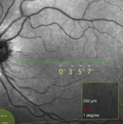
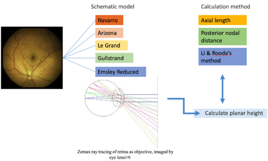
One problem in fundus photography arises from the very strong curvature of the retina and this problem increases with the field angle. The peculiarities of image formation in the optical system of a fundus camera makes it possible to focus the whole retina on a plane, maintaining the same image quality in the posterior pole as in the periphery. However, due to the fact that the human eye is also optical system, the unique eye structure of each individual, however, introduces different magnifications into the final retinal image so that the adaptive optics (AO) imaging always incorporates some assumptions of the eye structure into the calculation of this scale bar as shown in the figure on the left.

Retinal Magnification Factor

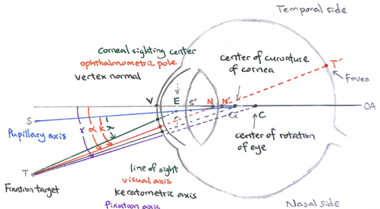
The retinal magnification factor (RMF) is defined as the paraxial height of the image (in mm) on the retina given a visual angle of 1°. As shown in Fig.3, the visual angle corresponds to the angle between the optical axis and the visual axis, which goes through the nodal points and joins the fixation target and the fovea of the eye. In this case of visual angle, in whatever angle that the rays enter the front nodal point of the system, they will come out at exactly the same angle from the rear nodal point. In general, there are two main geometrical lengths that need to be considered while calculating RMF: the axial length and the posterior nodal distance of the eye. (1) scaling RMF by the axial length (AL) is chosen by most of the lab groups; other groups choose to do the scaling based on (2) the back focal length (BFL) or the posterior nodal distance (PND) but they determine PND differently: (3) PND is linearly scaled based on PND of the Gullstrand-Emsley eye model, (4) PND is adjusted by the AL difference from Gullstrand-Emsley eye model, (5) PND is determined through paraxial raytracing with the measurement of the anterior chamber depth and curvature of the front cornea.

Fig.2 Important axis in the human eye

Fig.3 Schematic eye models. (a) Emsley reduced eye (b) Gullstrand-Emsley eye (c) Le Grand full theoretical eye (d) Gullstrand number 1 eye

Schematic Eyes

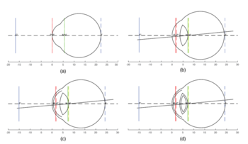
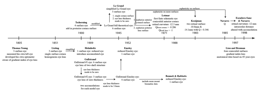
Schematic eyes are models that reveal human eye’s optical-related biometry.[1] They are useful in predicting and assessing the cardinal points of real eyes. The development of schematic eyes goes through several stages and the new models are largely based on the previous models. It generally derives into two main trajectories. The eye’s structure had been known since Johannnes Kepler in 1604. And in 1652, a century and a half before Young, Christiaan Huygens had come up with a ‘simplified eye’ consisting of a single spherical refracting surface separating air from water, forming an image onto another spherical surface with three time the radius. In 1909, Allvar Gullstrand came up with a six-refracting-surface model, which is known as Gullstrand’s number 1 eye (Fig.3d). The two-layer structure of the lens, which divides a single lens into outer cortex and core shells is based on the awareness of eye lens’ gradient index property.[2] In 1945, Le Grand presented a three-refracting-surface full theoretical eye (Fig.3c), a modification of the Tscherning schematic eye. Gullstrand also proposed a Gullstrand’s number 2 eye, which is a three-refracting-surface model but with a zero-thickness eye lens. In 1952 Emsley constructed the Gullstrand-Emsley eye (Fig.3b) by adding the 3.6mm thick lens into Gullstrand’s number 2 eye. Bennett and Rabbetts (1988) and Rabbetts (2007) modified Gullstrand-Emsley eye based on more recent biometric data.[1] The equivalent powers of the eye and crystalline lens changes from 58.64D to 60.00D and from 19.11D to 20.83D respectively.[3] In addition to the Gullstrand-Emsley eye, Emsley also proposed a more simplified model eye with only one refracting surface (Fig.3a).

Fig.4 Timeline of development of schematic eyes.

Methods

Paraxial Regime Ray Tracing

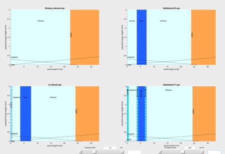
Fig.5 shows the MATLAB interface to ray trace light through the four classical schematic eye models using the ABCD matrix method, which is a method of tracing of a light path through the system by multiplying this matrix multiple vector representing the light ray bending and transferring.

Fig.5 Paraxial ray tracing with ABCD matrix method in MATLAB with different schematic eyes

Fig.6 RMF value for four schematic eye models based on adjusted axial length method

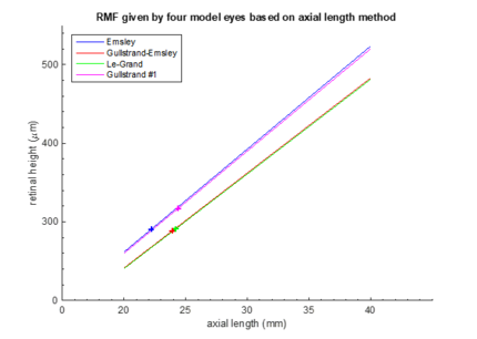Fig.6 gives RMF resulted from this method but based on the four different schematic eyes, i.e. different axial length is chosen as the reference. RMF determination depending on Emsley and Gullstrand No.1 eye models appears to be similar; same applies to RMF calculation based on Le-Grand full eye model and Gullstrand-Emsley, but with a more gradual slope. The discrepancy between the two main performance is about 8.40% with fixed axial length. However, this ABCD matrix analysis is limited to only the paraxial region. For region that's further away from the paraxial regime, we perform PBRT simulation.

PBRT Simulation for Extended Field

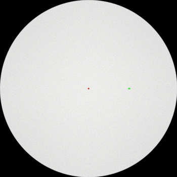
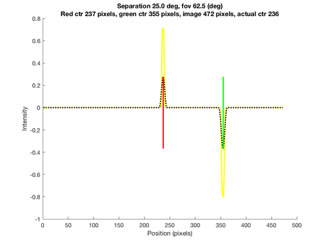
The Physically Based Rendering (PBRT) files are incorporated here into isetbio scenes and optical images. First of all, two spheres of known spatial separation in terms of visual angle with the same diameter but different colors are rendered on a blank scene. Then different schematic eye models are respectively written in as new lens files into 'SceneEye' (as accessible in SceneEye.m in Iset3d). The eye lens files are later passed into another file to enable accommodations of the eye. Here we adopted the model eyes at their relaxed form since during most AO imaging, patients are dilated in the darkness and their eyes are focused at infinity instead of a closer distance that requires accommodation. After the PBRT simulation is performed, we locate the positions of the peaks of the two sphere at the image plane. The image falls on a chord with specified width across the back of the spherical model eye. By accessing the pixel numbers covered in between the separation we are able to figure out the angular retinal height in mm and the main task is to convert the rendering from angular retinal height to planar height with Drasdo formula.

Fig.7 Initial rendered scene to calculate planar separation between the two color dots with known angular separation

Fig.8 Intensity of the scene vs pixel positions. This is used to locate the sphere separation by peak pixel intensity

Drasdo Formula

The 'Dacey and Petersen' method in the code is based on digitizing and fitting curves published by Drasdo and Fowler, where the tangential value was determined by the following equation: $T={\frac {11.06(sin5.181d)}{(57.3sin\theta )}}$, Where T is the tangential dimension corresponding to a coaxial arc length of 1° on retina, at a peripheral angle of \theta from the optic axis, and d is the eccentricity of the image point in millimeters of retinal arc. The area of the retina responsible for one solid degree angle at a given peripheral angle from the optical axis equals to the product of the retinal dimensions responsible for a radial and tangential degree. The data were then transformed to visual axis data by correction for angle alpha.[11] The table below shows the used Drasdo Fowler Data:

(deg)	(mm)
1.429393919263E0	4.001594366571E-1
3.492105671073E0	9.230850993158E-1
6.034234593326E0	1.662020859629E0
1.000354303683E1	2.739148342523E0
1.571668991785E1	4.215850660998E0
2.381363626298E1	6.400797183286E0
3.286388095396E1	8.862844615691E0
4.016364401337E1	1.073941407028E1
4.572178303328E1	1.227837640337E1
4.794503864125E1	1.289396133661E1
4.984831373591E1	1.335521158573E1
5.254323612126E1	1.396991961735E1
5.523705130760E1	1.455364379194E1
6.126021391085E1	1.590582608118E1
6.632675657123E1	1.688795588919E1
7.012555636750E1	1.759356938816E1
7.503155517173E1	1.848303992560E1
8.135698310414E1	1.949381518634E1
8.689076374588E1	2.035113266459E1
9.321065568325E1	2.120698864014E1
9.921278150535E1	2.197047764565E1];

Results

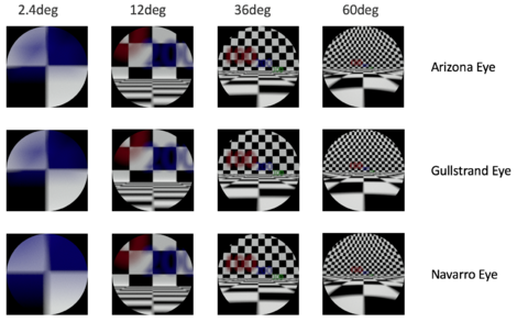
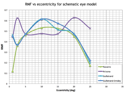
Fig.9 gives the simulation of the "Numbers at Depth" scene through multiple model eyes. Within the paraxial regime, which is around 0° to 3° here, the retinal magnification factor (RMF) changes linearly with the deviation angle away from the fovea axis. Starting from 3°, the nonlinear relationship between retinal magnification factor and visual angle is well shown in Fig.10. The non-linear behavior follows the predication by Draso and Fowler but gives more details from each specific eye model.

Fig.9 Example scene simulation with PBRT through different eye models. Field of field is varied from 1.2 to 36deg.

Fig.10 Simulated retinal magnification factor vs eccentricity within different eye models.

Conclusions

Due to the fact that the human eye is also optical system, the unique eye structure of each individual introduces different magnifications into the final retinal image so that the adaptive optics (AO) imaging always incorporates some assumptions of the eye structure into the calculation of this scale bar. The schematic eyes are modified for each individual eye by scaling the entire schematic eye or only portion of it based on the axial length of the particular eye being imaged. Most RMF calculation methods call the parameters of axial length or posterior nodal distance, one method incorporates also corneal curvature and anterior chamber depth measurements through paraxial ray tracing, which applies to pupil sizes less than 0.5mm and field angles less than 2°. As RMF estimation varies 8.40% using different schematic eyes and even with the same schematic eye, using different methods give maximum difference of 11.03%. The nonlinear relationship between retinal magnification factor and visual angle is well shown in Fig.10. As going away from the paraxial region, the projection of the visual field in the retinal area tends to become non-linear. In order to obtain a relatively accurate scale bar for the AO fundus image, we can adopt PBRT simulation and load in schematic eyes, together with utilizing the mapping from angular to planar retinal height with Drasdo formula to calculate RMF. Furthermore, it is even possible to construct and import customized patient's eye from the measured parameters using ophthalmoscopes so that each scale bar is more accurate and precise. This will greatly help with follow-up exams and patient's data comparison across different AO labs.

Future Work

More accurate estimations of the retinal magnification factors can be obtained through the following pipeline: treat the curved retina as the imaging object by rendering an fundus image on the sphere, flip the eye models so that we can analyze the final image at the cornea plane and how much the planar image height differ from different schematic model eyes.

Fig.9 simulation.

Reference

1. Atchison, D. ‘Schematic eyes, Handbook of Visual Optics’, Handbook of Visual Optics, 2017
2. Atchison, D. ‘Possible errors in determining axial length changes during accommodation with the IOLMaster’, Optometry and vision science, 2004, 81, (4), pp. 283-286
3. Bennett, A.G., Rudnicka, A.R., and Edgar, D.F.: ‘Improvements on Littmann's method of determining the size of retinal features by fundus photography’, Graefes Arch Clin Exp Ophthalmol, 1994, 232, (6), pp. 361-367
4. Li, K.Y., Tiruveedhula, P., and Roorda, A.: ‘Intersubject variability of foveal cone photoreceptor density in relation to eye length’, Invest Ophthalmol Vis Sci, 2010, 51, (12), pp. 6858-6867
5. Vakkur, G.J., Bishop, P.O., and Kozak, W.: ‘Visual Optics in the Cat, Including Posterior Nodal Distance and Retinal Landmarks’, Vision Res, 1963, 61, pp. 289-314
6. Bedggood, P., Daaboul, M., Ashman, R., Smith, G., and Metha, A.: ‘Characteristics of the human isoplanatic patch and implications for adaptive optics retinal imaging’, J Biomed Opt, 2008, 13, (2), pp. 024008
7. Escudero-Sanz, I., and Navarro, R.: ‘Off-axis aberrations of a wide-angle schematic eye model’, J Opt Soc Am A Opt Image Sci Vis, 1999, 16, (8), pp. 1881-1891
8. B. N. Behnken, G. Karunasiri, D. R. Chamberlin, P. R Robrish, and J. Faist,”Real-time imaging using a 2.8~THz quantum cascade laser and uncooled infrared microbolometer camera,”' Opt. Lett. 33(5), 440–442 (2008).
9. Muthiah MN, Gias C, Chen FK, et al Cone photoreceptor definition on adaptive optics retinal imaging British Journal of Ophthalmology 2014;98:1073-1079
10. http://stanford.edu/class/ee367/Winter2017/Tong_Melanson_ee367_win17_report.pdf
11. Dacey, D M and M R Petersen. 'Dendritic field size and morphology of midget and parasol ganglion cells of the human retina' Proceedings of the National Academy of Sciences of the United States of America vol. 89,20 (1992): 9666-70.

Appendix

Fig.10 Schematic eye model parameters.[1]

MATLAB Code:

isetbio>isettools:File:Utilities sceneeye zx.zip
iset3d:File:SceneEye zx.zip