Stephanie
Background
Recognition Memory
Several models of recognition memory hypothesize that the probability of judging a test-probe as “old” is correlated with the similarity between the test-probe and studied items stored in memory. For instance, these models claim that as the congruence between test-probe and studied items increases, the activation level for that probe will increase, and consequently it becomes more likely that test-probe will be judged as familiar (Gillund and Shiffrin, 1984; Hintzman, 1988). In the present experiment (Olsen, 2009), we sought to examine the neural correlates of recognition memory using functional magnetic resonance imaging (fMRI). More specifically, we used a novel set of abstract shape stimuli to manipulate the perceptual similarity between test-probes and studied items, allowing us to directly test the assumptions of these recognition memory models.
Highpass filtering
Temporally filtering fMRI data can be useful in cleaning up the raw signal. Given a priori estimates about how quickly the signal should be oscillating back and forth (i.e., the temporal cycle of the task), it can be useful to remove noise that is oscillating slower than the expected frequency. For instance, slow (i.e., low frequency) scanner drift, basal metabolism, or many other sources can cause raw fMRI signal to drift over the course of a session. In order to remove these low-frequency trends, one can highpass filter the data, filtering out the low frequencies while "passing through" the high frequencies (i.e., the frequencies related to the task of interest; see Fig. 1).

In order to remove the low frequency noise, one must first determine a highpass frequency cutoff (HPFC) parameter. This parameter can either be specified in Hz or in seconds. In FSL, the HPFC parameter is specified in seconds; this corresponds to the period of interest from the experiment. That is, frequencies that are lower (i.e., occurring over a period longer than the period of interest) will be removed, whereas higher frequencies are retained. After the design matrix is constructed, the highpass filter is applied to each individual voxel's timecourse before the model estimation takes place. Essentially, this highpass temporal filtering uses a local fit of a straight line (Gaussian-weighted within the line to give a smooth response) to remove low frequency artifacts.
Materials and Methods
Subjects
Subjects were 19 healthy, right-handed volunteers. All participants were native English-speakers, had normal or corrected-to-normal hearing and vision and had no history of psychiatric, neurological or memory disorder. Informed consent was obtained in a manner approved by the Stanford University IRB. Subjects were paid $60 for their participation in the study.
Memory Task
Subjects completed 12 scanned runs consisting of an encoding phase and a recognition test phase (see Fig. 2). Each encoding phase lasted 4.5 minutes, and the test phase lasted 1.5 minutes; separating the encoding and test phases was a delay period during which subjects performed an odd/even judgment task as a baseline condition.
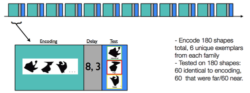
During a given encoding phase, subjects were presented with 15 unique shapes. Each of the 15 shapes was presented three times for 2.5 s each time (separated by a 1.5s ISI, during which a fixation was presented). Subjects were tasked with making a size judgment (i.e., aspect ratio; taller than wide, or wider than tall) for every shape.
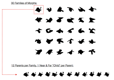
For each test phase, subjects were presented with 15 shapes (2.5 s duration, 1.5 s fixation); critically, five of the shapes were identical to the studied shapes, five were perceptually near shapes ("near"), and five were perceptually far ("far"). These shape stimuli were designed to yield 30 families of 12 exemplars, each of which had a near and far morph (see Fig. 3 for the 30 families, and 12 example exemplars). For each of the 15 shapes, subjects were asked to rate if the shape was new or old, using a 1-5 confidence rating scale (1:sure new, 2:moderately sure new, 3:guess, 4:moderately sure old, 5:sure old).
fMRI Analysis
MR acquisition
Imaging data were acquired on a 3.0 T Signa whole-body MRI system with a custom-built head coil (GE Medical Systems, Milwaukee, WI, USA).
In total, 2,400 functional volumes were acquired for each participant using a T2*-sensitive gradient echo spiral in/our pulse sequence (Glover and Law, 2001). Functional imaging parameters were optimized to provide whole brain coverage (TR=2000ms; TE= 30ms; flip angle = 75°; FOV = 22 cm; 3.44 x 3.44 x 4 mm resolution, 30 slices).
fMRI Analysis
The fMRI data was analyzed using Lyman, Nipype, Freesurfer, AFNI, and FSL software tools.
Preprocessing
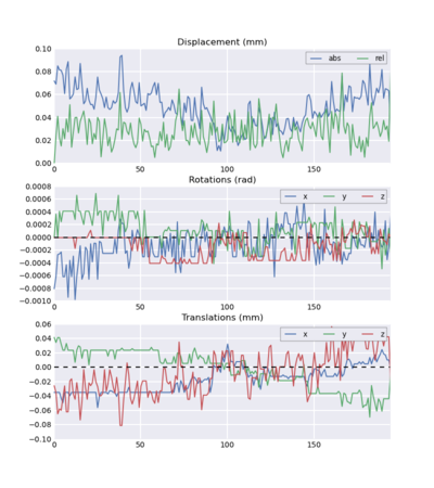
All data went through a standard preprocessing pipeline using Freesurfer and FSL, including motion (RapidART) and slice time correction, realignment (middle volume of each run), skull stripping, temporal filtering (high-pass cutoff 200 s, 128 s (as is standardly used in our lab), 30 s, 10 s), and surface-based coregistration (bbregister). Data were spatially smoothed (6 fwhm, SUSAN -- only averages a given voxel with local voxels that have a similar intensity), scaled grand median of timeseries to 10000, & normalized for group analyses (nonlinear warp to FSL’s MNI152 space). Data were modeled using a double gamma function, and the first 5 frames of each run were discarded.
Results
Behavioral Results
Perceptual similarity
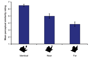
First, 2 separate groups of subjects rated the perceptual similarity between the different morphs used during the recognition test phase (1-7 scale, 1=least similar to 7=most similar). In general, subjects rated the identical morphs as very perceptually similar to the same morph. Further, subjects rated the near morphs as being more perceptually similar to the parent morph than they rated the far morphs; however, the near morphs were accurately judged to be less perceptually similar to the parent morphs than the identical morphs (see Fig. 4).
Recognition Memory
As predicted, recognition memory confidence was modulated by the perceptual similarity of the test morphs to the parent morph presented during encoding. That is, as the similarity between the test morph and the studied morph increased, recognition confidence ratings increased. Here, a repeated measures ANOVA comparing the mean recognition confidence scores across test morph type (identical: M=4.14, near: M=3.58 and far: M=2.72) found a significant effect of test morph similarity on recognition confidence ratings (F(92.14, p < 0.001). Paired comparisons between identical vs. near and near vs. far also revealed significant differences between recognition for these morphs (ps < 0.001).
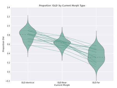
For the fMRI analyses, due to the relatively small number of trials in each condition/response bin, we coded trials as "OLD" if the subject had responded with a recognition confidence rating of 4 or 5 (moderately sure or sure old). Likewise, we coded trials as "NEW" if the subject had responded with a recognition confidence rating of 1 or 2 (moderately sure or sure new). Here, analyses confirmed that subjects rated a higher proportion of identical morphs as "OLD." Moreover, on average subjects rated more than half of the near morphs as "OLD." In general, the proportion of morphs rated as "OLD" decreased as the perceptual similarity between the test morph and the encoded parent shape decreased (identical > near > far; see Fig. 5).
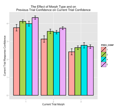
Further, based on recent findings from Duncan & Davachi (2012), we were interested in whether a subject's recognition confidence on a given trial might be modulated by their response confidence on the preceding trial. In other words, if a subject rates a morph as "confident old," might they then be more likely to rate the next morph as old? In addition, we were curious whether this effect might be modulated by the current trial morph, and it's similarity with the encoded shape (i.e., identical, near, far). To investigate this, we binned each trial based on the current morph type (i.e., identical, near, far), and the response confidence on the previous trial (i.e., OLD: 4,5 or NEW: 1,2). Here, we used a linear mixed effects model (LMM) predicting recognition confidence on the current trial, with the current morph type and previous trial confidence as fixed effects, random intercepts for subjects, and random slopes by morph type and previous trial confidence. As hypothesized, we found a significant effect of previous trial confidence (beta = 0.10, t=3.10), and no interaction (p>0.05), such that response confidence on the previous trial influences response confidence on the current trial regardless of the current trial morph type (see Figure below).
fMRI Results
For these fMRI analyses, we will report results from four iterations through the data. In each case, data preprocessing and the overall models were kept the same, varying only the highpass filter cutoffs. Here, we selected four unique cutoffs: 200, 128, 30, and 10 seconds. Based on calculations set to optimize highpass filtering (i.e., minimizing the period for the highpass filter that still preserves a specified amount of variance in all the design matrix regressors; FSL's cutoffcalc function), the optimal HPFC for this study ranged from approximately 114 to 222 seconds, with sigma bounds around 20-30. From these calculations, we should expect that highpass filter cutoffs lower than ~100 seconds would remove some task-related variation in signal, rather than just low-frequency noise.
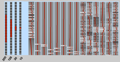
Model parameters across all four iterations of highpass frequency cutoffs included study trials (regardless of the repetition number, or subsequent recognition confidence), and test trials were separated by whether the response confidence was old (rating of 4 or 5) or new (rating of 1 or 2), a guess (rating of 3), by morph type (identical, near, far).
Single Subject Results
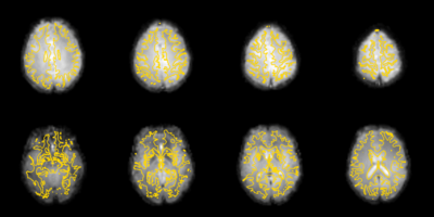
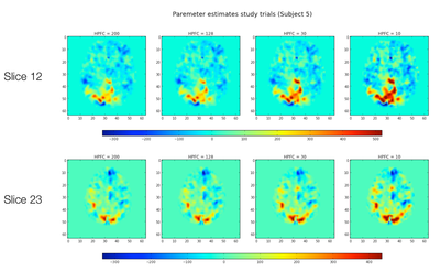
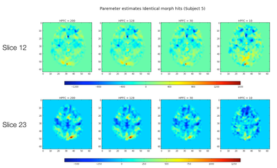
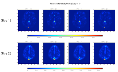
First, for a single subject we calculated the parameter estimates and residuals for "study" trials for one run, across the four different HPFCs using fixed effects within subjects across runs.
T-Statistics
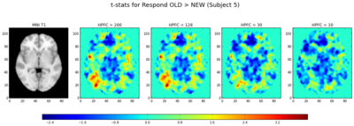
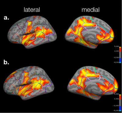
We also calculated the t-statistics (a linear combination of the parameter estimates, divided by the variance) for the contrasts of (1) Study > Test and (2) Responding OLD > Responding NEW (collapsing across morph types). In general, the t-statistics decrease as the highpass frequency cutoff decreases, as shown in Figures 9a and 10.
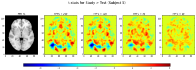
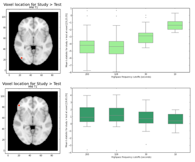
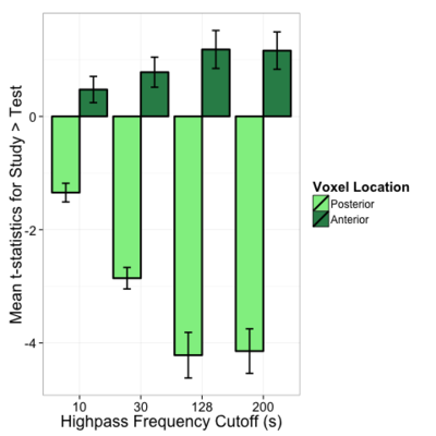
Interestingly, looking at the t-statistics at a single voxel averaged across subjects for the 4 different highpass frequency cutoffs, voxels that had significant negative statistics for study > test (i.e., higher activation for test trials), such as the posterior voxel [23,23,35], showed an increase in t-statistics as the highpass frequency filter cutoffs were lowered; similarly, an anterior voxel [19,83,35] with more positive t-statistics for study > test demonstrated the opposite trend, such that the t-statistics tended to decrease as the HPFC was lowered (Fig. 9b and 9c). In both cases, the contrasts became less significant for HPFCs of 30 and 10. A repeated measures ANOVA examining the effect of highpass frequency cutoff (10, 30, 128, 200 seconds) and voxel location (anterior, posterior) on the mean t-statistic indicated significant main effects of HPFC (F(1,18) = 20.86, p < 0.001] and voxel location [F(1,18) = 77.23, p < 0.001], but importantly, there was a significant interaction between highpass frequency cutoff and voxel location for this dataset [F(1,94) = 72.54, p < 0.001], such that the main effect of highpass frequency cutoff was only marginal for the anterior voxel (p=0.06), but was significant for the posterior voxel [F(1,18) = 43.06, p < 0.001]. It might be interesting to investigate this more in depth to see whether the effect of highpass frequency filter cutoffs is differential for other anterior/posterior voxels, and whether this might generalize across tasks.
Group Results: Varying the Highpass Filter Cutoffs
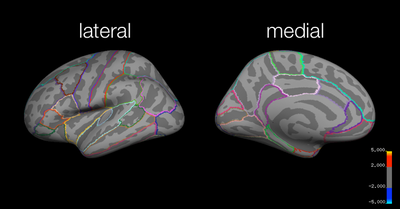
Group results were analyzed with a mixed effects analysis using FSL and Lyman, taking into account the within-subject fixed effects variances across runs, and the between-subject random effect variance. Data were normalized to MNI space. All inflated surfaces are displayed with a z-threshold of 2.3 to 4.265.
Study > Test
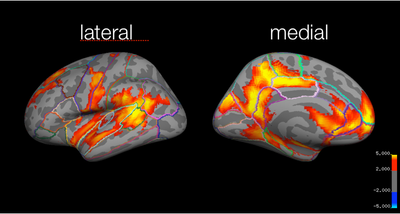
Local maxima estimates (200 HPFC): 
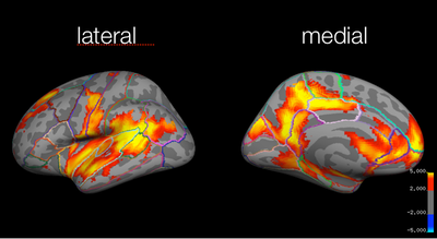
Local maxima estimates (128 HPFC): 
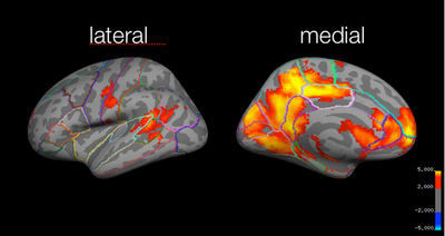
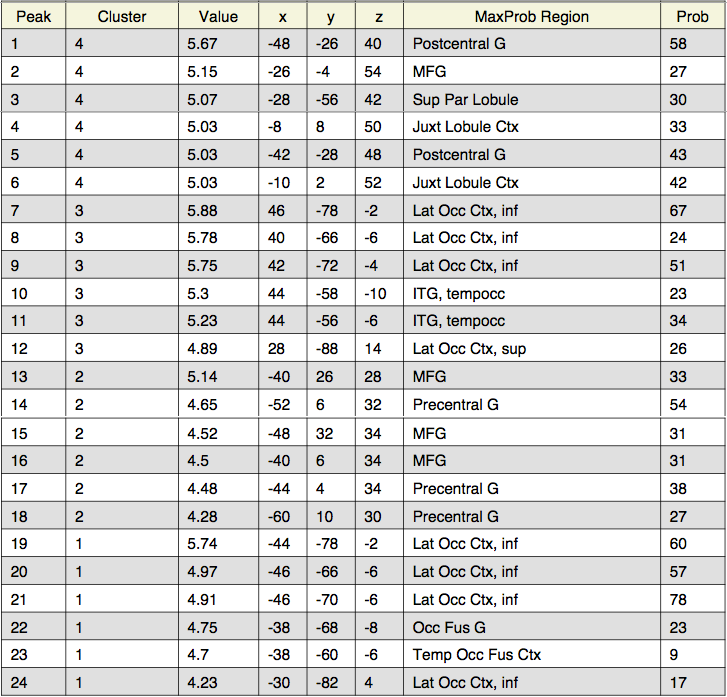
Local maxima estimates (30 HPFC): 
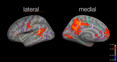
Local maxima estimates (10 HPFC): 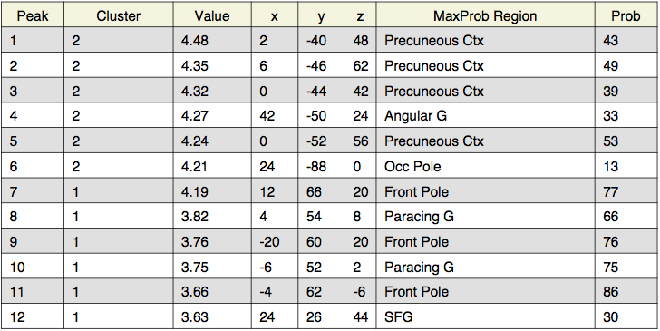
Test:Identical > Test:Far
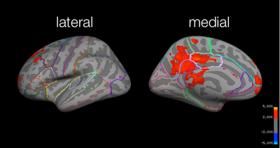
Local maxima estimates (200 HPFC): 

Local maxima estimates (128 HPFC): 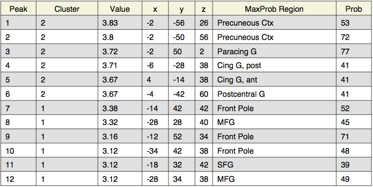
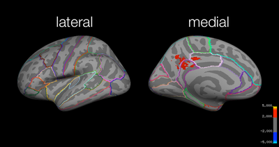
Local maxima estimates (30 HPFC): 
Group Results: Additional Analyses
Test > Study
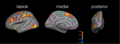
Using 2 unique fixed parameters in a model (coding for study and test trials), we investigated how learning the shapes (i.e., study trials) differed from retrieving information about the shapes (i.e., test trials, collapsing across response confidence and morph type) for the 128 HPF cutoff data.
Study > Test
For the Study > Test contrast using the simple coding for test trials (i.e., collapsing across all types of morphs and recognition confidence), the pattern of activation is essentially the same as the coding of test trials mentioned above, although the cluster significance increases slightly. Moreover, the superior frontal & dorsal rostral prefrontal activation observed before is no longer significant.
Conclusions
In summary, when the highpass frequency cutoff is lowered below 100 seconds (i.e., 30 or 10 seconds), the parameter estimates are decreased, and the t-statistics also decrease. Extending the temporal period of interest to 200 seconds did not seem to effect the results much; however, when data with temporal periods over 10 or 30 seconds was filtered out, the results changed significantly. Here, for the group analyses, the z-statistics decrease with lower highpass frequency cutoffs. For instance, for the study > test contrast, the highest probability precuneus cluster had a z-value of 6.48 for the 128s filter, but only 4.35 for the 10s filter. Similarly, for the identical > far test morph contrast, the frontal activation was below threshold for the 30s filter, and all activation was below threshold for the 10s filter.
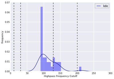
This pattern of results was predicted by using FSL's cutoffcalc function, which can be used to estimate an ideal highpass frequency cutoff (removing the low frequency trends elicited by non-task related drift, but also sufficiently long to avoid removing the signal of interest) based on the design matrices; for the present experiment, the mean estimated cutoff was 112.63 seconds, with a standard deviation of 25.57 (see Fig. 21). In summary, when choosing a highpass frequency cutoff one should carefully consider the temporal period of the design matrix to ensure that the filtering does not remove signal related to the task.
References
Gillund, G., & Shiffrin, R. M. (1984). A retrieval model for both recognition and recall. Psychological Review, 91, 1-67. [1]
Hintzman D (1988) Judgments of frequency and recognition memory in a multiple-trace memory model. Psychological Review 95:528-551. [2]
Olsen, R.K. (2009). Study-test visual similarity affects behavioral and neural correlates of recognition memory. Dissertation. [3]
MIT's MindHive: [4]
Duncan K., Sadanand A., & Davachi L. (2012). Memory’s penumbra: Episodic memory decisions induce lingering mnemonic biases. Science, 337(6093), 486-487. [5]
FSL's FMRI Expert Analysis Tool (FEAT) [6]
