WanlingLiuQianDong

Introduction

Image deblurring is an important task in the area of image processing and computer vision. The goal of image deblurring is to recover a sharp image for a blurry image. Motion blur, which happens when there is a relative motion between a camera and a scene during the image exposure time, is a common source of blurring when we take photos. We can reduce the effect of undesirable motion blur by reducing exposure time, and it is a fairly straightforward way to solve the problem. However, this method can increase image noise significantly especially in dark scenes. We can also use ISP (image signal processor) to deblur image, though the conventional ISP pipeline solves certain subproblem at each step and requires certain engineering work (refer to Fig. 1). Algorithms dealing with deblurring commonly set various constraints to model the blur, and those constraints limit the generalization of the model (i.e. when in real life, the blur is more complex, and the model can fail). Sometimes fine-tuning model parameters is also an issue since it may need a certain level of prior knowledge.

Due to the complexity of designing traditional approaches, people are trying to use machine learning to deal with those problems. Machine learning is able to learn and remove the blur without knowing prior information (e.g. kernel functions). In this project, we study and find robust machine learning methods for blind motion deblurring. There are two kinds of blurry images, one is blind images, knowing the sharp images while not knowing the source of blurring, and the other one is non-blind, knowing both the sharp image and blurring source. We focus on the blind images in our project. To address the blurry image problem, CNN (convolutional neural network) and GAN (generative adversarial network) are commonly used. For example, [1] used a multi-layer perceptron (MLP) for non-blind images, [2] designed a deep multi-scale CNN for dynamic scene deblurring, and [3] applied GAN for blind images. Therefore, we mainly focus on these two kinds of models and by comparing their pros and cons, we choose the model with the best performance and robustness. Furthermore, we combine and modify the existing model to boost the performance of the models. We calculated MSE (Mean Square Error), PSNR (Peak Signal to Noise Ratio), SSIM (Structural Similarity) and S-CIELAB (spatial CIELAB) to evaluate our results. Our dataset is the GOPRO dataset [2], which is widely used for training and testing the models for motion deblurring. The dataset can be found here.

Dataset

We use the GOPRO dataset [2]. The dataset contains 3214 pairs of blurry and sharp images at 1280x720 resolution and is publicly available at this website. We randomly selected 2103 images as our training set and 500 images as our testing set (training set: testing set $\approx$ 8:2).

As for the generation of image pairs, they adopted kernel-free methods for generating blurry images, which is to approximate the camera imaging process instead of designing complex kernels. They used GOPRO4 Hero Black camera to take 240 fps videos, averaging (integrating, more details are described in section 2 of [2]) various number (7-13) of successive latent frames to produce different strengths of blurs (the motions are caused by both camera shake and object movement). The sharp image corresponding to each blurry image is defined as the mid-frame among sharp images used to produce blurry images.

Methods

ISP

The traditional way to process image and signal is to use ISP tools. Process related with deblurring is commonly based on the evaluation of the point spread function and noise in the image. Algorithms are used to find the blur kernel and then recover the blurry image to the original image. In real circumstances, there would not be enough information for finding the blur kernel. Therefore, traditional deblurring methods are easy to suffer from intensive parameter tuning and poor performance.

Fig. 1 ISP pipeline (credit: Zheng Lyn)

GAN model

GAN structure

A generative adversarial network is a popular deep learning approach to generate new realistic images. The architecture is comprised of a pair of competing generators and discriminator. The generator learns how to generate plausible fake images that ideally are indistinguishable from real examples in the dataset. The discriminator model is trained to classify whether a given image is real(real-world images) or fake(generated images). By competing with each other, the two models grow together and finally, we will have a good generator and discriminator.

Fig. 2 Conditional generative adversarial network architecture.

Different generator architectures

• Simple generator

A simple generator is comprised of a downsampling encoder and an upsampling decoder. Both networks are based on convolutional networks typically one or two convolutional layers following by a maxpooling layer.

Fig. 3 The generator architectures used in Pix2Pix[1]

• U-net-based generator

U-net [6] is a convolutional neural network which was developed for image segmentation at first. The architecture is still based on the standard convolutional neural network, but with the internal connection between encoder and decoder, the modified generator is extended to smaller datasets.

• VGG16-based generator

Fig. 4 VGG16-based generator architecture [2]

To accelerate the GAN converging speed and reduce the overfit due to a limited dataset, the encoder of the generator is replaced by a pretrained VGG16 with all parameters locked for transfer learning. Based on the architecture, the time for each epoch is only half of the U-net generator and it also converges much earlier than U-net generator.

CNN model

• SRN (scale-recurrent network) structure

Fig. 5 SRN-DeblurNet framework [4]

Xin Tao et al. proposed the scale-recurrent network (SRN) which is shown in Fig. 5. There are five basic modules that are worth noticing:

1. Encoder-decoder: this is adapted from U-net [6]. This structure improves the network’s regression ability and is widely used in image and video processing.

2. Residual Block: [7] proposed a structure that has an additional shortcut (identity mapping) connection compared with conventional structure that stacks layers. This structure can deal with the gradient vanishing problem [7] and is useful for deep networks.

3. Skip connection: skip connection is used for combining different levels of features and also good for gradient flow and accelerating convergence.

4. Scale connection: the model can benefit from scale connection since the scale connection makes it possible for the model to train for different scales of images, solving the problem of overfitting specific scales.

5. RNN: at each scale level, we are doing similar work, therefore, we can use RNN to connect different levels. The characteristics of RNN is to share weights between each hidden state, which has the effect of reducing parameters to decrease the risk of overfitting and increasing efficiency.

• Modified model

Fig. 6 Our basic block

Though Tao et al. proposed the SRN model, they also discussed the influence of RNN layers and they suggested that without using RNN, the model can still generate comparable results. Therefore, we decided to modify the SRN model by removing the RNN layers and change their basic block to further simplify the model and explore the potential of pure CNN. As shown in Fig. 6, our block also stacks convolutional layers and has the basic structure of residual module but would be computationally cheaper. In general, this simplified model combines the advantages mentioned in the previous section and further improves efficiency.

Image Quality Evaluation

MSE

The mean-square error computes the pixel-based difference between two images which represents the cumulative squared error between the deblurred and the original image. A lower value of MSE represents a lower error and a high image quality.

$MSE={\frac {1}{mn}}\sum _{i=0}^{m-1}\sum _{j=0}^{n-1}[I(i,j)-K(i,j)]^{2}$

PSNR

PSNR is the ratio between the maximum possible value (power) of a signal and the power of distorting noise that affects the quality of its representation. The ratio can be used as a reference for image quality evaluation between the original and the deblurred image. An image with a higher PSNR has a higher image quality.

$PSNR=10\log _{10}({\frac {MAX_{I}^{2}}{MSE}})$

SSIM

SSIM is used for measuring the structural similarity between the two images. SSIM is designed to improve the evaluation metrics of images such as peak signal-to-noise ratio (PSNR) and mean squared error (MSE).

$SSIM(x,y)={\frac {(2\mu _{x}\mu _{y}+C_{1})+(2\sigma _{xy}+C_{2})}{(\mu _{x}^{2}+\mu _{y}^{2}+C_{1})+(\sigma _{x}^{2}+\sigma _{y}^{2}+C_{2})}}$

The above three metrics above are commonly used for evaluating the quality of deblurring. Combining those three metrics we expect they can offer a general trend about the quality of results from the aspects of pixel-based difference, noise level, and structural difference. However, those parameters do not include much information related to human perception. Therefore, we investigated more about the metrics.

S-CIELAB

We also use S-CIELAB [5] to evaluate different models. S-CIELAB merges CIELAB and human spatial sensitivity and provides a difference between a reference and a corresponding test image. The calculation step is shown in Fig. 8. For the S-CIELAB error measurement, the first step is to implement spatial filtering to the image data which simulates the human visual system, and then, the calculation is consistent with the basic CIELAB calculation.

Fig. 8 A flow-chart for S-CIELAB computation.[5]

Yolo object detection

Yolo object detection network [3] is one of the most popular networks for the object detection task. The algorithm is based on a neural network and can detect all the objects on the image. The network divides the image into grids and output detected objects with bounding boxes and confidence. Since Yolo object detection is trained based on real people object detection, it can be used to justify where the image quality is increased. A better quality image is supposed to increase objects detected and detection confidence.

Fig. 7 Yolo object detection block [3]

Results

GAN

As for runtime consideration, we used 256x256 images for the preliminary experiments.

• Model comparison

Model Comparison (averaged data for 100 epochs on the test set)
Model	Blurry Image	GAN with Unet generator	GAN with VGG16 generator
MSE	227.90	289.19	361.49
PSNR	24.55	23.52	22.55
SSIM	0.79	0.74	0.72
S-CIELAB	672	1209	1485
Runtime (s/epoch)	N/A	375.71	163.67
Trainable parameters	N/A	54,414,979	13,753,091

The table above compares the deblurring performance of two GAN models by analyzing MSE, PSNR, SSIM, S-CIELAB, runtime and trainable parameters. The result shows that the deblurred images generated by two models are worse than the original blurry images. The main reason is even though the GAN models serve the function of deblurring, they generate too much noise and artifacts. The GAN model with pretrained VGG16 network has less trainable parameters and shorter runtime but it suffers more from the artifacts. The reason will be further analyzed in the later section.

• Example image results

Model Comparison (100 epochs on the sample image)
Model	Blurry Image	GAN with Unet generator	GAN with VGG16 generator	Sharp image
MSE	222.75	337.44	415.21	N/A
PSNR	25.75	23.44	22.50	N/A
SSIM	0.79	0.77	0.74	N/A
S-CIELAB	755	1003	1623	N/A
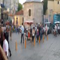
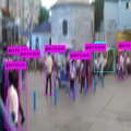
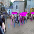
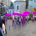
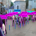
Objects detected	18	13	13	22
Detection Confidence	75%	82.23%	79.92%	82.77%

• 

  Blurry Image

• 

  GAN with U-net

• 

  GAN with VGG16

• 

  Sharp Image

• 

  Blurry Image(Object detection)

• 

  GAN with U-net(Object detection)

• 

  GAN with VGG16(Object detection)

• 

  Sharp Image(Object detection)

The table and the figures above show the comparison between the two models based on the example images. Consistent with the comparison results for the test set, the GAN model with VGG16 generator produce worse results than GAN with U-net generator, and those results are worse than the original blurry images.

• GAN model analysis

Even though the generated images by GAN look much sharper, they suffer from the problems of artifacts and noises. After thoroughly analyzing our results, we find that the GAN model has some common issues which make them not suitable for our application.

1. Non-convergence: The generator and discriminator compete with each other during the training and the model parameters oscillate instead of keeping going down. This model is hard to be trained to converge.
2. Mode collapse: The generator collapses which produces limited varieties of samples. Since our dataset is not that large, the GAN model may not be a good choice.
3. Unbalance training between the generator and discriminator can cause overfitting.

CNN

We compared our preliminary CNN's result with GAN's result:

Fig. 9 CNN vs. GAN

As shown in Fig. 9, though GAN's result image is less blurry than what CNN produced, there are many artifacts in GAN's image. Considering the metrics calculated in the previous section, GAN is not even better than the original blurry image. For practical consideration, we decided to focus on CNN and conducted more experiments with images of higher quality (original size 1280x720) to explore the deblurring effect of CNN.

• Different CNN models

We compared the results produced by Tao's CNN model (without using recurrent network) [4] and our modified model:

Model Comparison (averaged data for 100 epochs on the test set)
Model	Blurry Image	Tao et al.	Ours
MSE	222.75	190.48	162.91
PSNR	25.75	26.35	27.04
SSIM	0.785	0.793	0.816
S-CIELAB (e+04)	3.72	2.93	2.43
Runtime (s/epoch)	N/A	245	187

We can see from the table above that both Tao's model and our model improve the quality of the original blurry image. Our model leads to more improvement compared with Tao's model and our runtime is also shorter. Some examples are shown below to visually compare those results:

• 

  Blurry Image

• 

  Tao's Result (100 epochs)

• 

  Our Result (100 epochs)

• 

  Our Result (300 epochs)

• 

  Sharp Image

• 

  Blurry Image

• 

  Tao's Result (100 epochs)

• 

  Our Result (100 epochs)

• 

  Our Result (300 epochs)

• 

  Sharp Image

• 

  Blurry Image

• 

  Tao's Result (100 epochs)

• 

  Our Result (100 epochs)

• 

  Our Result (300 epochs)

• 

  Sharp Image

We can see from the examples above that our model produced deblurred image with higher quality compared with Tao's CNN model: the qualitative metrics (MSE, SSIM, PSNR and S-CIELAB) of our model are better and the images also looks clearer (for better comparison, please refer to the images of full resolution). Examples in the second row suggests that our model is able to recover most of the information even when the blurry image suffers from severe motion blur. It is also interesting to notice the characters (marked with a red rectangle) in the images in the third row. At first, it is hard for us even to guess the characters in the blurry image, but after the image being processed by our model, we are able to read those characters.

• 

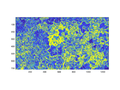
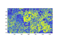  Spatial Distribution of Errors for Blurry Image 1

• 

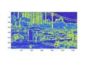
  Spatial Distribution of Errors for Blurry Image 2

• 

  Spatial Distribution of Errors for Blurry Image 3

• 

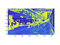
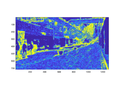
  Spatial Distribution of Errors for Deblurred Image 1

• 

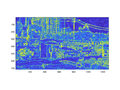
  Spatial Distribution of Errors for Deblurred Image 2

• 

  Spatial Distribution of Errors for Deblurred Image 3

Figures above show the spatial distribution of the errors of S-CIELAB for <blurry image, image deblurred by our model (300 epochs)> pairs. We can conclude that our model is able to reduce much error and thus has better image quality (lower S-CIELAB difference with the sharp image) and the errors are mostly located around the edges.

• CNN vs. ISP

For comparison, we utilized two ISP tools pinetools and SmartDeblur to test the result.

Fig.10 Example 1: a. blurry image (from Internet); b. result of our model; c. result of pinetools; d. result of SmartDeblur

Fig.11 Example 2: a. blurry image (from Internet); b. result of our model; c. result of pinetools; d. result of SmartDeblur

For both examples, results produced by pinetools are more blurry than what our model produced. The results produced by SmartDeblur look sharper, but there are many artifacts (e.g. change of color) and more noise. Those behaviors of ISP tools are predictable since their algorithms are designed to deal with the edge intentionally and they model the blur with some restrictions which would introduce some artifacts when the blur is complex. It is also worth noting that ISP tools often requires complex tuning of parameters and the results depends greatly on those parameters, which is not very friendly for those without much experience in image processing.

Discussion

• We implemented two machine learning models, GAN and CNN and our CNN model performs better than the GAN model. However, we only tried one specific GAN model with U-Net generator and VGG16 generator, and there can be other GAN models that may work better for deblurring.

• The evaluation metrics we used (MSE, PSNR, SSIM, object detection, S-CIELAB) in general indicate the trend, though sometimes they have limitations when compared with what humans perceive.

• The images produced by our current CNN model are clearer but not perfectly deblurred especially for high-frequency parts (edges, fine details, etc.). The reason can be that due to the time and budget limitation (our CNN model was trained in the NVIDIA Tesla P100 GPU), the model has not converged yet and we expected the output would be more desirable if we train our model for more epochs. The other reason is that the current loss function only takes content loss (multi-scale Euclidean loss [4]) into account, which can be improved by including perception loss like S-CIELAB. We expected that the model performance would be boosted especially when dealing with high-frequency data. We can also design a better architecture that works for sharpening edges.

• When dealing with deblurring, we can notice that for images showing the effect of depth-of-field (DOF), the deblurring model would not influence on the DOF effect, which is a nice characteristic since the DOF effect is what we want to preserve (see Fig. 10 and Fig. 11). This also suggests that our model is practical for real-life usage.

Conclusion

In this project, we compared traditional methods with machine learning methods, and for machine learning approach, we tried several models. ISP tools often need complex parameter tuning process and would introduce more noise and artifacts, while CNN models are more straightforward to use and produce images of good quality. Compared with Tao's CNN model, our CNN model is computationally cheaper and yields better results. Generally speaking, our model is able to produce competitive and practical results in a reasonably fast time (though the training time for our model is long, the testing time is very short which means we can deblur images quickly after training on some dataset).

Reference

[1] Schuler, C. J., Christopher Burger, H., Harmeling, S., & Scholkopf, B. (2013). A machine learning approach for non-blind image deconvolution. In Proceedings of the IEEE Conference on Computer Vision and Pattern Recognition (pp. 1067-1074).

[2] Nah, S., Hyun Kim, T., & Mu Lee, K. (2017). Deep multi-scale convolutional neural network for dynamic scene deblurring. In Proceedings of the IEEE Conference on Computer Vision and Pattern Recognition (pp. 3883-3891).

[3] Kupyn, O., Budzan, V., Mykhailych, M., Mishkin, D., & Matas, J. (2018). Deblurgan: Blind motion deblurring using conditional adversarial networks. In Proceedings of the IEEE Conference on Computer Vision and Pattern Recognition (pp. 8183-8192).

[4] Tao, X., Gao, H., Shen, X., Wang, J., & Jia, J. (2018). Scale-recurrent network for deep image deblurring. In Proceedings of the IEEE Conference on Computer Vision and Pattern Recognition (pp. 8174-8182).

[5] Zhang, X., & Wandell, B. A. (1996, May). A spatial extension of CIELAB for digital color image reproduction. In SID international symposium digest of technical papers (Vol. 27, pp. 731-734). SOCIETY FOR INFORMATION DISPLAY.

[6] Ronneberger, O., Fischer, P., & Brox, T. (2015, October). U-net: Convolutional networks for biomedical image segmentation. In International Conference on Medical image computing and computer-assisted intervention (pp. 234-241). Springer, Cham.

[7] He, K., Zhang, X., Ren, S., & Sun, J. (2016). Deep residual learning for image recognition. In Proceedings of the IEEE conference on computer vision and pattern recognition (pp. 770-778).

Acknowledgment

Thank Professor Brian Wandell for sharing the insight related with the depth of field, Dr. Joyce Farrell for the advice of metrics, and Zheng Lyu for discussing the loss functions and project idea.

Appendix I: Code

Github Page: https://github.com/lwlynn/Psych221_CourseProject.git

Appendix II: Contributions

Wanling Liu: CNN models, ISP tools, model evaluation, writing the report

Qian Dong: finding the dataset, GAN models, model evaluation, writing the report