Wavefront optics toolbox

^{Back to Psych221-Projects-2012}

We worked with the WavefrontOpticsToolbox, located in a SVN repository at https://platypus.psych.upenn.edu/repos/toolboxes/WavefrontOpticsToolbox/trunk. This toolbox models the optics of the human eye using scalar diffraction theory from Fourier optics. In particular, the aberrations of the human cornea, pupil, and lens, as well as the Stiles-Crawford effect from retinal cone cells, are modeled by the amplitude and phase of the eye's pupil function. This pupil function is then Fourier transformed to compute the eye's point spread function (PSF).

The project is split into two sections: 1) code clean-up and commenting and 2) the creation of a MATLAB tutorial to demonstrate some of the features of the toolbox.

• 

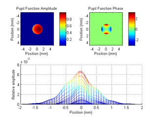
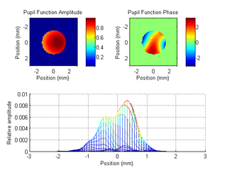  One subject's eye data: (top) Amplitude and phase of the pupil function, (bottom) xz view of the PSF.

• 

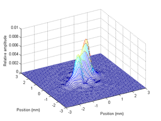  3D view of the same subject's PSF.

Background

Ray optics, or geometric optics, is concerned with modeling how light rays travel through optical systems like that of our eyes. However, to fully consider the effects of small pupil size, as well as variations in the geometry and chromatic aberrations of the eye's lenses, wave optics and diffraction must be accounted for. Fourier optics, or scalar diffraction theory, cleanly handles effects such as wavefront aberrations, finite pupil size, and apodizing filtering, so we will first briefly give a background of Fourier optics. Next, we will discuss how wavefront aberrations are modeled, namely by the basis set of Zernike polynomials. Finally, we will describe the Stiles-Crawford effect, the physical cause of this effect, and how it is modeled.

Fourier optics

Huygens-Fresnel principle

Fourier optics is built upon the idea that the wave nature of light is modeled by the Huygens-Fresnel principle -- that every point on a wavefront of light is the source of new spherical waves. The summed interaction of these spherical waves at some observation plane determines what is observed at that plane. Here, it is assumed that the polarization of the electromagnetic field can be neglected, and instead, light can simply be modeled by a wavefunction that obeys the standard wave equation and represents electric or magnetic field. Hence, this is called scalar diffraction theory.

A direct result of this theory is that the diffraction effects of any imaging system can be modeled very cleanly by Fourier transforms. In fact the point spread function of an imaging system is given by [1]

$h(u,v)={\frac {A}{\lambda z_{i}}}\iint \limits _{-\infty }^{\infty }\!P(x,y)\exp \left\{-j{\frac {2\pi }{\lambda z_{i}}}(ux+vy)\right\}\,\mathrm {d} x\,\mathrm {d} y$

where $A$ is a constant amplitude, $\lambda$ is the wavelength of monochromatic light, $z_{i}$ is the distance from the exit pupil to the image plane, $P(x,y)$ is the pupil's complex transmittance function, $(u,v)$ are image coordinates, and $(x,y)$ are coordinates in the pupil plane. Thus, we can see that the PSF is just the Fraunhofer diffraction pattern, or Fourier transform, of the exit pupil. The intensity actually observed on the retina is $|PSF|^{2}$.

The expression above has several consequences for modeling the PSF of the human eye. First, it handles monochromatic light, so in order to obtain the polychromatic PSF, the equation above must be computed for several (or many) wavelengths of light. Secondly, care must be taken to sample $P(x,y)$ finely enough to avoid aliasing; the phase of this function must be slowly varying at the chosen sampling rate. In addition, care must be taken to pad $P(x,y)$ with enough zero values to avoid "ringing" effects associated with the periodic boundary conditions of the discrete Fourier transform.

Diffraction-limited PSF and the eye

The pupil function $P(x,y)$ of a diffraction-limited optical system is simply given by [1]

$P(x,y)=\mathrm {circ} \left({\frac {\sqrt {x^{2}+y^{2}}}{w}}\right)$

where $\mathrm {circ} (\rho )$ is 1 for $\rho \leq 1$ and 0 for $\rho >1$, $r^{2}=x^{2}+y^{2}$, and $w$ is the radius of the pupil.

Airy disk

The Fourier transform of a circular pupil is the so-called Airy disk, given by [1]

$U(r)=\exp(jkz)\exp \left(j{\frac {kr^{2}}{2z}}\right){\frac {A}{j\lambda z}}\left[2{\frac {J_{1}(kwr/z)}{kwr/z}}\right]$

where $k=2\pi /\lambda$, $z$ is the distance from the pupil to the retina, and $J_{1}$ is a Bessel function of the first kind.

Here, the diffraction-limited pupil function is a real function that has uniform amplitude. However, there are two effects in human eyes that make their PSFs non-ideal. The first is wavefront aberrations caused by distortions of the cornea, pupil, and lens of the eye. These are modeled by a complex phase function $W(x,y)$ that modifies the pupil function. The second arises from the waveguide-like nature of the cone cells in the retina, which only capture light over a limited angular range. This is modeled by a amplitude variation $A(x,y)$ in the pupil function. Thus, in general, we can model the complex pupil function as

$P(x,y)=A(x,y)\exp \left[jkW(x,y)\right]\mathrm {circ} \left({\frac {\sqrt {x^{2}+y^{2}}}{w}}\right)$

Wavefront aberrations and Zernike polynomials

Zernike polynomials $Z_{n}^{m}$ in pyramid arrangement

As stated above, wavefront aberrations are modeled by phase variations in the pupil function. In order to conveniently describe the different types of aberrations that occur, The Optical Society has developed a standard convention [2] based upon the complete basis set of Zernike polynomials. These polynomials are orthogonal over the unit circle $\rho \leq 1$. They are indexed either by a pair of numbers $(n,m)$ or by their overall mode number $j$. The radial order $n$ specifies the power of the radial portion of the polynomial, while the angular frequency $m$ specifies the number of angular nodes. For each radial order $n$, there are $n+1$ polynomials forming a pyramid structure. To make indexing more convenient, especially when computing these functions in software, the single index $j=\left[n(n+2)+m\right]/2$ is widely used and adopted here.

Since the polynomials form a complete orthogonal basis set over the unit disk, the wavefront aberrations of any human eye can be decomposed into the basis of Zernike polynomials:

$W(x,y)=\sum \limits _{j=0}^{\infty }z_{j}Z_{j}\left(\rho ={\frac {\sqrt {x^{2}+y^{2}}}{w}},\theta =\mathrm {atan2} (y,x)\right)$

Thus, it is sufficient to express the wavefront aberrations of any pupil function with a series of Zernike coefficients $z_{j}$.

Notable polynomials and their aberration names are given below.

Zernike polynomial	Aberration name
$Z_{0}(\rho ,\theta )=1\!$	Piston
$Z_{1}(\rho ,\theta )=2\rho \sin \theta \!$	$y$ tilt
$Z_{2}(\rho ,\theta )=2\rho \cos \theta \!$	$x$ tilt
$Z_{3}(\rho ,\theta )={\sqrt {6}}\rho ^{2}\sin 2\theta$	Primary astigmatism at $45^{\circ }$
$Z_{4}(\rho ,\theta )={\sqrt {3}}\left(2\rho ^{2}-1\right)$	Defocus
$Z_{5}(\rho ,\theta )={\sqrt {6}}\rho ^{2}\cos 2\theta$	Primary astigmatism at $0^{\circ }$
$Z_{7}(\rho ,\theta )={\sqrt {8}}\left(3\rho ^{3}-2\rho \right)\sin \theta$	Primary $y$ coma
$Z_{8}(\rho ,\theta )={\sqrt {8}}\left(3\rho ^{3}-2\rho \right)\cos \theta$	Primary $x$ coma
$Z_{12}(\rho ,\theta )={\sqrt {5}}\left(6\rho ^{4}-6\rho ^{2}+1\right)$	Primary spherical

Stiles-Crawford effect

The Stiles-Crawford effect arises from the tall waveguide-like nature of cone cells. Reported in 1933 by W.S. Stiles and B.H. Crawford [3], light impinging on the retina invokes different responses in cone cells based upon the incident angle. In the pupil plane, this suggests that rays entering the center of the pupil more efficiently excite photoreceptors compared to rays entering the edges of the pupil. Although this effect is strictly retinal in nature, it is modeled by an attenuating filter on the pupil function. It is hypothesized that this effect improves vision by decreasing the cone's response to aberrated or scattered light, especially since phase aberrations are worse near the edges of the pupil.

The model of the Stiles-Crawford effect is an exponentially decaying amplitude function [4]

$A(x,y)=\exp \left\{-\alpha \left[(x-x_{0})^{2}+(y-y_{0})^{2}\right]\right\}$

where $\alpha =0.116\pm 0.029$ is an apodization factor and the peak location of transmission is given by $(x_{0},y_{0})=(0.47\pm 0.68,0.20\pm 0.64)\mathrm {mm}$.

Toolbox code clean-up

One of the goals of the wavefront optics toolbox is to help students understand and explore the use of Zernike polynomial representations of pupil functions and PSFs. To this end, the toolbox had to undergo some changes in order to to expose its associated functions with more transparency. This included the addition of comments explaining the use of subfunctions or parameters where applicable, rewriting functions so that their computation and output is more obvious, and restructuring wavefront variable parameters in a more physically meaningful way.

Comments

Zernike coefficients vector

wvfCreate.m and wvfSet.m form a 65-element column vector of "Zernike coefficients." For clarity, these have been explained as the weights of the first 65 terms of the Zernike polynomials, representing up to 10 orders of these basis functions. These terms follow the "j" single-indexing scheme adopted by OSA. [2]

Nominal wavelength and Defocus

It was previously unclear what the purpose of the nominal (in-focus) wavelength was. We have made it clear that computing a pupil function for a wavelength other than the nominal wavelength under which the Zernike coefficients were measured must account for longitudinal chromatic aberration (LCA). This is the result of the optics of the eye focusing light at different points on-axis depending on wavelength. With the exception of the 4th coefficient, "defocus," aberrations do not vary much with wavelength. As a result, the toolbox adjusts for LCA by introducing it into the "defocus" coefficient. wvfComputePSF.m uses wvfGet to provide a defocus value in microns (because Zernike coefficients are in units of microns). Within wvfGet, this is done by calling wvfGetDefocusFromWavelengthDifference.m, a utility function which first converts the difference between the nominal and calculated-for wavelengths into diopters. It then combines this with any user-preset defocus in diopters. Finally, it converts all contributions to defocus from diopters into microns using the referenced equation. [5] The defocus in microns is finally set as the 4th term of the vector of Zernike coefficients on a wavelength by wavelength loop to compute the pupil function and PSF.

Code edits

Wavelength vector inputs

wvfSet.m can now accept a vector of wavelengths over which the pupil function and PSF are computed, specified in the format: [start spacing Nsamples]. The PSF will change if not being calculated for the nominal wavelength due to longitudinal chromatic aberration (LCA) effects, so it is useful to store multiple PSFs for multiple wavelengths at once using this format.

Removal of unnecessary loops

Previously, the Stiles-Crawford Effect (SCE) and Zernike polynomial computations of pupil function amplitude and phase, respectively, were handled in nested for loops for all x and y points in the specified field. This method was not only cumbersome, but also did not clearly reflect the natural conversion between polar and rectangular coordinate systems, which is one of the benefits of using the Zernike polynomials as the set of basis functions in the first place. We use the simple relations:

$x=r\cos \theta \,$

$y=r\sin \theta \,$

$Rnorm={\sqrt {y^{2}+x^{2}}}/MeasuredPupilRadius\quad$

$\theta =\operatorname {atan2} (y,x)\quad$

This allowed us to initialize columns of x values and rows of y values in a matrix of pupil positions. From there, the contribution of each Zernike polynomial to the phase for each $(x,y)$ pupil position could be summed up in vectorized form using their original normalized radius and theta coordinates.

Additional plotting functionality

We have included additional switch cases to wvfPlot.m so that it can plot the amplitude and phase of pupil functions over space parameters (in units of mm). While these are unintuitive out of context, which is why the toolbox exists to convert Zernike coefficients into a more intuitive PSF representation, they serve a useful purpose in the tutorial. The pupil functions can be used to visualize the Zernike polynomial basis functions themselves, allowing students to see the independent impact of each coefficient on a pupil function.

Parameter Restructuring

Physical units for specifying field size

The Wavefront optics toolbox creates wavefront variables in a struct format using wvfCreate, wvfSet, and wvfGet to create, set, and retrieve wavefront parameters such as nominal wavelength and measured pupil size. Previously, there were two complementary parameters for setting the field over which the pupil function, and eventually the PSF, were computed and generated for plots: sizeOfFieldPixels and sizeOfFieldMM. In the toolbox functions, however, these two parameters were very ambiguously defined and it was unclear that they were both required to set field matrices rather than alternative ways of doing so. Additionally, while sizeOfFieldMM has specified units, sizeOfFieldPixels was only used to set the number of sample pixels, and this use of "pixels" in other functions lacked physical meaning out of context. We have therefore changed the parameters to sizeOfFieldMM, like before, and fieldSampleSizeMMperPixel. The new parameter fieldSampleSizeMMperPixel specifies a sampling rate in millimeters/pixel for the field size (given in mm) from the other parameter. The associated functions automatically determine the necessary number of pixels based on this size and sampling rate. This will hopefully carry more physical meaning throughout the Wavefront toolbox and help in understanding what the functions do. It is still possible to derive the number of pixels using the simple relation that $Npixels=sizeOfFieldMM/fieldSampleSizeMMperPixel$.

Tutorial

In addition to cleaning up and commenting the wavefront optics toolbox so that it is more understandable, we have also created a tutorial for students to learn about the Zernike polynomials and explore the functionality of the toolbox.

Zernike polynomials

The first section of the tutorial is devoted to explaining the background of using the Zernike polynomials as the set of basis functions for approximating measured eye aberrations. This includes going over the 65-element vector of "j" single-indexed Zernike polynomial weighting coefficients. This is done in part by comparing a zero vector (which corresponds to an un-aberrated pupil function, and therefore a diffraction-limited point-spread function) to vectors with one non-zero element. This also shows how the Zernike polynomials are useful for breaking down a complex PSF into individual categorizable aberrations.

Here is an example showing how the tutorial generates a diffraction-limited PSF and a PSF with a non-zero weight on the 3rd coefficient, which corresponds to "astigmatism at 45 degrees," as explained in the background above. We show the code here to give a feel for calling wavefront toolbox functions. Comments and explanations that were present in the tutorial have been removed for this.

Zcoeffs = zeros(65,1);

wvf0 = wvfCreate

wvf0 = wvfComputePSF(wvf0);

vcNewGraphWin;

maxMM = 1;

wvfPlot(wvf0,'2dpsf space normalized','mm',maxMM);

Zcoeffs(3) = 0.75;

wvf3 = wvfSet(wvf0,'zcoeffs',Zcoeffs);

wvf3 = wvfComputePSF(wvf3);

vcNewGraphWin;

maxMM = 2;

wvfPlot(wvf3, '2d psf space normalized','mm',maxMM);

• 

  All-zero coefficients, Diffraction-Limited PSF.

• 

  Non-zero weight on 3rd coefficient, Astigmatism at 45 degrees.

Modeling chromatic aberration

The next section of the tutorial shows how chromatic aberration can change the PSF. The wavefront toolbox variables can be set with a nominal focus wavelength at which the measured Zernike coefficients correspond to an eye in focus. But the toolbox can also calculate PSFs which would occur for non-nominal wavelengths and thus model chromatic aberration. Through a series of examples, we show that since wavefront aberrations are generally independent of wavelength (with the exception of the "Defocus," the 4th Zernike coefficient), the toolbox automatically converts any effect of chromatic aberration into a defocus value (in units of microns like Zernike coefficients) and combines it into the 4th term of the Zernike coefficients vector. This both explains the optical principle and elucidates how the toolbox functions handle it.

Below we show the plot generated in this section of the tutorial, which compares the 1D PSF slices of:

(1) all-zero coefficients/diffraction-limited PSF (narrower red line);

(2) two identical ways of representing a chromatically aberrated PSF: one by changing the nominal focus wavelength such that we are measuring the PSF for a non-nominal wavelength (wider red line), the other by adding a defocus in microns to Zernike coefficients vector as calculated from the same difference in wavelengths by a wavefront toolbox function (thin blue line).

• 

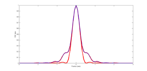  Illustration of chromatic aberration modeling in the wavefront toolbox. Diffraction-limited PSF (red) and chromatically-aberrated PSF (red/blue).

Stiles-Crawford effect

In this part of the tutorial we explain an additional factor introduced into the computation of the pupil function. While the complex exponential representing the pupil function gets its phase from the weighting of Zernike polynomials, its amplitude comes from the Stiles-Crawford effect. This amplitude term is itself a decaying exponential which attenuates the pupil function at the edges of the pupil, but relative to an off-axis center (as explained in the Stiles-Crawford effect section). The tutorial demonstrates how the SCE actually helps improve the PSF in some cases, as the edges of the pupil function often contain the most severe phase aberrations, and this is where the SCE does its attenuation.

Below we see the Stiles-Crawford effect (SCE) in practice and improvements in the PSF. On the left we have the pupil function amplitude and phase, as well as the resulting PSF, for a wavefront with the only non-zero weight on the 5th Zernike coefficient (Astigmatism along the XY axes). The amplitude function is constant since the SCE has not been applied. On the right we have the pupil function amplitude and phase, as well as the resulting PSF, for the same aberrated wavefront, but with the SCE applied this time. The amplitude function shows attenuation near one edge of the pupil function. In the PSF we see that this translates to a reduced width, albeit asymmetrically.

• 

  Astigmatism along XY axes without SCE: (top) Amplitude and phase of the pupil function, (bottom) xz view of the PSF.

• 

  Astigmatism along Xy axes with SCE: (top) Amplitude and phase of the pupil function, (bottom) xz view of the PSF, showing asymmetrical PSF narrowing.

Human eye aberrations and correction using eyeglasses

In the final part of the tutorial, we explore the aberrated wavefront measurements of real human eyes. We show the amplitude, phase, and resulting PSFs for a few different eyes in order to note the apparent complexity of the aberrations and the highly asymmetric PSFs. This is how each point of light is blurred for us! But now that we have an understanding of how Zernike polynomials work, we can see that these complex aberrations can actually be decomposed into various categorized aberrations of different orders. The weighting coefficients of lower-order Zernike polynomials are particularly noteworthy, because they represent the aberrations that are commonly corrected for by using single-vision eyewear.
These terms include:

Zernike coefficient (4) & (6) - Astigmatism along 45 degrees and 0 degrees, respectively, which create asymmetric blurring

Zernike coefficient (5) - Defocus, the typical myopic or hyperopic blurring that +/- diopter power in lenses correct

Below is the data for one subject's eye, which is provided entirely in a 65-element vector of Zernike polynomial weighting coefficients. On the left is the uncorrected pupil function and PSF for the eye. On the right we have simulated eyeglass correction by zeroing out the 3rd through 5th coefficients, thus removing the contribution of the two astigmatism terms and defocus to the phase of the pupil function. The resulting PSF is clearly narrower (will blur less) and is much more symmetrical.

• 

  One subject's eye data: (top) Amplitude and phase of the pupil function, (bottom) xz view of the PSF.

• 

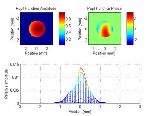  Same subject's eye data, but with defocus and astigmatism coefficients set to zero, simulating eyeglass correction: (top) Amplitude and phase of the pupil function, (bottom) xz view of the PSF.

Conclusions and future directions

Revisions to the Wavefront Optics Toolbox are still incomplete. One prominent issue that remains is how wvfComputePSF.m still attempts to scale the calculated PSF relative to the scaling that an arbitrary reference wavelength would produce (by default, 550nm). This comes from taking the Fourier Transform of the pupil function and is not a feature of the Zernike polynomials. Rewriting this portion of the code is important not only because it is confusing and not intuitive, but because it affects the resulting plots. Since the toolbox functions and associated tutorial are meant to be explored by students in order to understand pupil function and PSF computations, it would be much better to have a clearly-defined scaling based on a physical parameter in the code. With more time, this would be a natural and key next-step for the project.

Another potential area of development is the exploration of human eye data in the tutorial. Currently, there are Zernike polynomial coefficients for nine subjects. Each set, however, is missing the 4th Zernike polynomial coefficient (representing defocus), meaning we do not have a complete picture of the eye aberrations. The tutorial would be clearer and deeper with the addition of more complete human data matching the inputs that the toolbox already uses, for example, nominal focus wavelengths in wavefront aberration measurements and defocus diopters of the refractive power of eyes. With these data and a larger set of subjects, the tutorial could perhaps include some statistical analysis.

Finally, while the tutorial has explored the how pupil functions and PSFs can be changed by correcting certain aberrations, it would be beneficial to combine this with sample images to compare "before and after" vision correction. This would require scaling and sizing/distance computations in order to properly convolve different versions of the PSF with images for simulating their appearance.

References

1. Goodman, J. W. (2005). Introduction to Fourier optics. 3rd ed. Englewood, Colo.: Roberts & Co.
2. Porter, J. (2006). Adaptive optics for vision science: principles, practices, design, and applications (Appendix A: Optical Society of America's Standards for Reporting Optical Aberrations). Hoboken, NJ: Wiley-Interscience.
3. Stiles W. S. and Crawford B. H. (1933). "The luminous efficiency of rays entering the eye pupil at different points," Proc. R. Soc. Lond B 112:428-450.
4. Schwiegerling, J. (2004). Field guide to visual and ophthalmic optics. Bellingham, Wash.: SPIE.
5. Tarrant, J. (2010). Determining the accommodative response from wavefront aberrations. Journal of Vision.

Appendix I

Code

File:T Zernike.zip

WavefrontOpticsToolbox SVN repository

Data

Wavefront measurements of human eyes are part of the WavefrontOpticsToolbox SVN repository.

Presentation

File:2012LewPhong WaveOpticsToolbox.zip

Appendix II - Work partition

Matthew Lew - Heavily edited wvfComputePupilFunction.m to remove unnecessary nested loops; removed sizeOfFieldPixels field of the wvf struct so that all parameters are defined in terms of physical dimensions, not pixels; constructed sections of tutorial dealing with SCE and vision correction with eyeglasses

Kevin Phuong - Constructed core of t_Zernike.m to demonstrate Zernike polynomials and their effect on PSFs; updated various functions of the toolbox to use wvfGet() and wvfSet(); comments and references in wvfComputePSF.m and wvfGetDefocusFromWavelengthDifference.m.