David Gal: Difference between revisions
imported>Dgal1 No edit summary |
imported>Dgal1 No edit summary |
||
| Line 14: | Line 14: | ||
As a result of what has become “overkill” for the typical consumer researchers have begun to consider other uses of pixels in imaging sensors. One such utilization of the pixels on a sensor is the realization of novel color filter arrays (CFA). | As a result of what has become “overkill” for the typical consumer researchers have begun to consider other uses of pixels in imaging sensors. One such utilization of the pixels on a sensor is the realization of novel color filter arrays (CFA). | ||
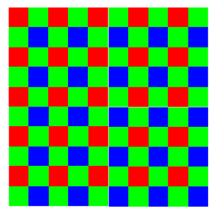
The ubiquitous Bayer pattern has served both the consumer and professional photographic community well. It’s design and consideration for the human visual system – namely high sampling of green wavelengths – has rendered it a universally accepted standard in still camera design. Numerous papers have been published on the Bayer pattern’s merits as well as algorithms for demosaicing, denoiseing, and color transforming its resultant sensor data. | The ubiquitous Bayer pattern seen in the figure below has served both the consumer and professional photographic community well. It’s design and consideration for the human visual system – namely high sampling of green wavelengths – has rendered it a universally accepted standard in still camera design. Numerous papers have been published on the Bayer pattern’s merits as well as algorithms for demosaicing, denoiseing, and color transforming its resultant sensor data. | ||
<br> | |||
[[File:Bayer Pattern.jpg | Figure 1 - Bayer Pattern]] | |||
The Bayer pattern is, however, not without its limitations and despite it’s universal adoption should by no means be considered the end all and be all of CFA design. Researchers have considered countless designs of CFA patterns in the past, but with the advent of such pixel rich sensors they may well find their way into the consumer market. One such considered improvement to CFA design is the addition of a “white” pixel in the array. Such a pixel would filter at near infrared frequencies and provide a true luminance channel. With this additional channel low-light photography could occur with faster shutter speeds thus reducing blur. Additionally it’s possible that higher dynamic range images could easily be captured. | The Bayer pattern is, however, not without its limitations and despite it’s universal adoption should by no means be considered the end all and be all of CFA design. Researchers have considered countless designs of CFA patterns in the past, but with the advent of such pixel rich sensors they may well find their way into the consumer market. One such considered improvement to CFA design is the addition of a “white” pixel in the array. Such a pixel would filter at near infrared frequencies and provide a true luminance channel. With this additional channel low-light photography could occur with faster shutter speeds thus reducing blur. Additionally it’s possible that higher dynamic range images could easily be captured. | ||
The trouble with novel CFA design is not, however, in the design of the array itself. It is in fact in the design – or rather lack of design – of the image-processing pipeline that transforms sensor data to an image on a screen. As aforementioned countless methods for demosaicing, denoising, and color transformation exist for the Bayer pattern, but for a novel CFA pattern there is no reason to assume such algorithms exist. The necessity of such algorithms can be a major bottleneck in novel CFA research. | The trouble with novel CFA design is not, however, in the design of the array itself. It is in fact in the design – or rather lack of design – of the image-processing pipeline that transforms sensor data to an image on a screen. As aforementioned countless methods for demosaicing, denoising, and color transformation exist for the Bayer pattern, but for a novel CFA pattern there is no reason to assume such algorithms exist. The necessity of such algorithms can be a major bottleneck in novel CFA research. | ||
| Line 24: | Line 28: | ||
L3 stands for local, linear, and learning. Indeed the L3 algorithm is all of these. There are two fundamental components to the L3 algorithm – a regression stage that builds libraries of filters and an application stage that utilizes these filters to perform image processing. | L3 stands for local, linear, and learning. Indeed the L3 algorithm is all of these. There are two fundamental components to the L3 algorithm – a regression stage that builds libraries of filters and an application stage that utilizes these filters to perform image processing. | ||
The regression stage involves taking several images with any CFA pattern at different illuminant levels. L3 categorizes 9 x 9 sections of an image known as patches into two fundamental types – flat patches and texture patches for smooth and edged surfaces respectively. Knowing what the ideal image should look like a novel regression algorithm creates an ideal filter set for various structural elements within an image. For every color element in the CFA pattern a filter library is created. In the case of a Bayer pattern there are four filter libraries – one for red, two for green, and one for blue. | The regression stage involves taking several images with any CFA pattern at different illuminant levels. L3 categorizes 9 x 9 sections of an image known as patches into two fundamental types – flat patches and texture patches for smooth and edged surfaces respectively. Knowing what the ideal image should look like a novel regression algorithm creates an ideal filter set for various structural elements within an image. For every color element in the CFA pattern a filter library is created. In the case of a Bayer pattern there are four filter libraries – one for red, two for green, and one for blue. Figure 2 shows the contents of a filter library. | ||
<br> | <br> | ||
[[File:FilterLib.jpg | Figure | [[File:FilterLib.jpg | Figure 2 - Filter Library for a Red Pixel]] | ||
As seen there are several different filters in a single library. All filters are applied using the standard correlation method (convolution without kernel flipping) as seen in equation N | As seen there are several different filters in a single library. All filters are applied using the standard correlation method (convolution without kernel flipping) as seen in equation N | ||
PUT IN EQUATION HERE | |||
The final filters – the flat and texture filters – must be applied to a patch that is rotated and transformed to be in a canonical layout with the darkest area of the patch in the upper left corner. Patches may be flipped horizontally, vertically, translated across the major diagonal, or some combination of these transformations. | The final filters – the flat and texture filters – must be applied to a patch that is rotated and transformed to be in a canonical layout with the darkest area of the patch in the upper left corner. Patches may be flipped horizontally, vertically, translated across the major diagonal, or some combination of these transformations. | ||
| Line 37: | Line 43: | ||
= Algorithm Analysis = | = Algorithm Analysis = | ||
Figure | Figure 3 graphically depicts the per patch algorithm utilized to give X, Y, Z color estimates at a given pixel. | ||
<br> | |||
[[File:AlgorithmBD.jpg | Figure 3 - Per Patch Algorithm]] | |||
As seen this algorithm is quite computationally intensive. For a 500 x 500 image there are at least 162 million floating point multiply accumulate operations. For a 3-megapixel image there are 2 billion floating point multiply accumulate operations. Clearly there are a proportional number of memory references as well. It should be noted that the algorithm actually scales relatively well. Adding, for example, more levels to the PCA tree does not significantly contribute to computational complexity. The largest contributor to computational complexity is, in fact, the size of the filter/patch pair. | As seen this algorithm is quite computationally intensive. For a 500 x 500 image there are at least 162 million floating point multiply accumulate operations. For a 3-megapixel image there are 2 billion floating point multiply accumulate operations. Clearly there are a proportional number of memory references as well. It should be noted that the algorithm actually scales relatively well. Adding, for example, more levels to the PCA tree does not significantly contribute to computational complexity. The largest contributor to computational complexity is, in fact, the size of the filter/patch pair. | ||
As Matlab is an interpreted environment such computational complexity can result in very slow algorithmic execution. A faster implementation would be useful for researchers interested in novel CFA patterns. | As Matlab is an interpreted environment such computational complexity can result in very slow algorithmic execution. A faster implementation would be useful for researchers interested in novel CFA patterns. | ||
= Towards a Faster Implementation = | = Towards a Faster Implementation = | ||
Figure | Figure 3 also indicates a huge amount of potential thread and data level parallelism, which Matlab is likely not exploiting. Such parallelism fits well within the modality of super-scalar processor architectures, but even more so with modern graphics processors (GPUs), which can be thought of multi-cored, threaded vector architectures. | ||
As a baseline reference a pure CPU implementation was realized utilizing C++ and the OpenCV libraries. As the L3 pipeline involves a large amount of matrix-based operations the OpenCV libraries, which are based on the BLAS libraries, were utilized in the implementation. OpenCV libraries are open source and are accompanied by relatively good documentation. | As a baseline reference a pure CPU implementation was realized utilizing C++ and the OpenCV libraries. As the L3 pipeline involves a large amount of matrix-based operations the OpenCV libraries, which are based on the BLAS libraries, were utilized in the implementation. OpenCV libraries are open source and are accompanied by relatively good documentation. | ||
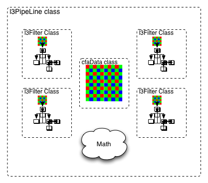
A three-class model was chosen for the implementation. As seen in Figure | A three-class model was chosen for the implementation. As seen in Figure 4 a cfaData class, l3Filter class, and l3PipeLine class were realized. | ||
<br> | |||
[[File:ClassModel.jpg | Figure 4 - Class Model of C++/OpenCV L3 Implementation]] | |||
The cfaData class contains: | |||
A matrix of sensor data | A matrix of sensor data | ||
| Line 72: | Line 88: | ||
The C++/OpenCV implementation of L3 is a promising first step in realizing a truly data and thread parallel implementation on a GPU. As compared to the Matlab implementation the C++/OpenCV implementation realized roughly a 6x speed up on average. On a macbook pro with a 2.5 GHz Core 2 Duo with 4 GB 667 MHz DDR2 SDRAM the average Matlab execution of a single L3 image was found to be 11.59 seconds compared to an average 2.06 seconds using the C++/OpenCV implementation. | The C++/OpenCV implementation of L3 is a promising first step in realizing a truly data and thread parallel implementation on a GPU. As compared to the Matlab implementation the C++/OpenCV implementation realized roughly a 6x speed up on average. On a macbook pro with a 2.5 GHz Core 2 Duo with 4 GB 667 MHz DDR2 SDRAM the average Matlab execution of a single L3 image was found to be 11.59 seconds compared to an average 2.06 seconds using the C++/OpenCV implementation. | ||
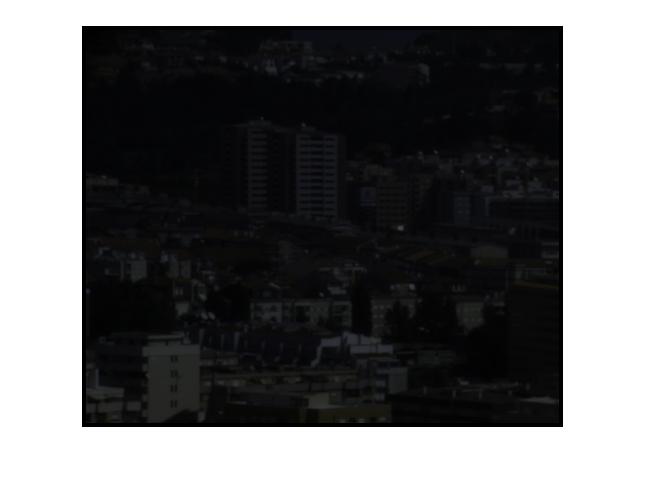
Figure | Figure 5 shows an output image from the C++/OpenCV implementation. | ||
<br> | |||
[[File:Output.jpg | Figure 5 - Example Output of C++/OpenCV L3 Implementation]] | |||
Utilization of the C++/OpenCV L3 implementation is trivial from the programmer’s perspective. Simply declare a new instantiation of an l3PipeLine and execute the process method: | Utilization of the C++/OpenCV L3 implementation is trivial from the programmer’s perspective. Simply declare a new instantiation of an l3PipeLine and execute the process method: | ||
Revision as of 08:58, 18 March 2011
Back to Psych 204 Projects 2009
Introduction
This project aims to realize a fast implementation of the novel L3 image-processing pipeline developed by Steven Lansel at Stanford University. Background
Background and Motivation
Moore’s law has resulted in unprecedented scaling of both the technology and economy of the semi conductor industry. Among other advancements, semi-conductor scaling has enabled CMOS imaging sensors to reach resolutions of 10s of millions of pixels (MegaPixels). Traditional research in imaging technology has often focused on improving key metrics of these sensors such as SNR, sensitivity, and cost. The abundance of pixels in today’s commercially available imaging sensors has become something of a marketing campaign and competition for leading camera manufactures. At present both Canon and Nikon offer consumer cameras with more than 20 million pixels. Given a monitor with 72 dots per inch (DPI) such cameras are capable of producing images that at full size occupy in excess of 60” in a single dimension. As a result of what has become “overkill” for the typical consumer researchers have begun to consider other uses of pixels in imaging sensors. One such utilization of the pixels on a sensor is the realization of novel color filter arrays (CFA).
The ubiquitous Bayer pattern seen in the figure below has served both the consumer and professional photographic community well. It’s design and consideration for the human visual system – namely high sampling of green wavelengths – has rendered it a universally accepted standard in still camera design. Numerous papers have been published on the Bayer pattern’s merits as well as algorithms for demosaicing, denoiseing, and color transforming its resultant sensor data.
The Bayer pattern is, however, not without its limitations and despite it’s universal adoption should by no means be considered the end all and be all of CFA design. Researchers have considered countless designs of CFA patterns in the past, but with the advent of such pixel rich sensors they may well find their way into the consumer market. One such considered improvement to CFA design is the addition of a “white” pixel in the array. Such a pixel would filter at near infrared frequencies and provide a true luminance channel. With this additional channel low-light photography could occur with faster shutter speeds thus reducing blur. Additionally it’s possible that higher dynamic range images could easily be captured.
The trouble with novel CFA design is not, however, in the design of the array itself. It is in fact in the design – or rather lack of design – of the image-processing pipeline that transforms sensor data to an image on a screen. As aforementioned countless methods for demosaicing, denoising, and color transformation exist for the Bayer pattern, but for a novel CFA pattern there is no reason to assume such algorithms exist. The necessity of such algorithms can be a major bottleneck in novel CFA research.
L3 Motivation and Background
The L3 pipeline developed by Steven Lansel aims to mitigate this bottleneck. The L3 pipeline is capable of performing demosaicing, denoising, and color transformation with the application of a single filter thus ameliorating the need for a novel pipeline for every novel CFA pattern.
L3 stands for local, linear, and learning. Indeed the L3 algorithm is all of these. There are two fundamental components to the L3 algorithm – a regression stage that builds libraries of filters and an application stage that utilizes these filters to perform image processing.
The regression stage involves taking several images with any CFA pattern at different illuminant levels. L3 categorizes 9 x 9 sections of an image known as patches into two fundamental types – flat patches and texture patches for smooth and edged surfaces respectively. Knowing what the ideal image should look like a novel regression algorithm creates an ideal filter set for various structural elements within an image. For every color element in the CFA pattern a filter library is created. In the case of a Bayer pattern there are four filter libraries – one for red, two for green, and one for blue. Figure 2 shows the contents of a filter library.
As seen there are several different filters in a single library. All filters are applied using the standard correlation method (convolution without kernel flipping) as seen in equation N
PUT IN EQUATION HERE
The final filters – the flat and texture filters – must be applied to a patch that is rotated and transformed to be in a canonical layout with the darkest area of the patch in the upper left corner. Patches may be flipped horizontally, vertically, translated across the major diagonal, or some combination of these transformations.
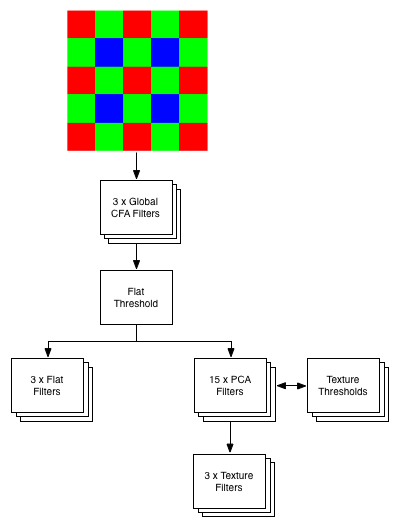
The three Weiner filters known as Global CFA filters are utilized to give a rough estimate of the patch type – either texture or flat. If a patch is determined flat then the three flat filters give estimates for X, Y, and Z. If a patch is determined to be textured then N PCA filters are utilized to determine the texture type. In the case of this project there are 16 texture types. The PCA filters are organized in a binary tree fashion such that only 4 PCA filters need to be applied to determine the ultimate texture type. Finally the appropriate texture filters can be applied to give estimates in X, Y, Z color space. In its current iteration the L3 pipeline is implemented entirely in Matlab.
Algorithm Analysis
Figure 3 graphically depicts the per patch algorithm utilized to give X, Y, Z color estimates at a given pixel.
As seen this algorithm is quite computationally intensive. For a 500 x 500 image there are at least 162 million floating point multiply accumulate operations. For a 3-megapixel image there are 2 billion floating point multiply accumulate operations. Clearly there are a proportional number of memory references as well. It should be noted that the algorithm actually scales relatively well. Adding, for example, more levels to the PCA tree does not significantly contribute to computational complexity. The largest contributor to computational complexity is, in fact, the size of the filter/patch pair.
As Matlab is an interpreted environment such computational complexity can result in very slow algorithmic execution. A faster implementation would be useful for researchers interested in novel CFA patterns.
Towards a Faster Implementation
Figure 3 also indicates a huge amount of potential thread and data level parallelism, which Matlab is likely not exploiting. Such parallelism fits well within the modality of super-scalar processor architectures, but even more so with modern graphics processors (GPUs), which can be thought of multi-cored, threaded vector architectures. As a baseline reference a pure CPU implementation was realized utilizing C++ and the OpenCV libraries. As the L3 pipeline involves a large amount of matrix-based operations the OpenCV libraries, which are based on the BLAS libraries, were utilized in the implementation. OpenCV libraries are open source and are accompanied by relatively good documentation.
A three-class model was chosen for the implementation. As seen in Figure 4 a cfaData class, l3Filter class, and l3PipeLine class were realized.
The cfaData class contains:
A matrix of sensor data A texture map matrix A flip map matrix Functions to load sensor data and parameter from Matlab generated text files
The l3Filter class contains:
3 x Global CFA filters 1 x Flat threshold 3 x Flat Filters 15 x PCA filters 15 x Texture thresholds 16 x 3 Texture Filters Methods to load filter data and parameters from Matlab generated text files
The l3PipeLine class contains:
1 x cfaData 4 x l3Filter Methods to process the pipeline and output Matlab read text files with results
Results
The C++/OpenCV implementation of L3 is a promising first step in realizing a truly data and thread parallel implementation on a GPU. As compared to the Matlab implementation the C++/OpenCV implementation realized roughly a 6x speed up on average. On a macbook pro with a 2.5 GHz Core 2 Duo with 4 GB 667 MHz DDR2 SDRAM the average Matlab execution of a single L3 image was found to be 11.59 seconds compared to an average 2.06 seconds using the C++/OpenCV implementation.
Figure 5 shows an output image from the C++/OpenCV implementation.
Utilization of the C++/OpenCV L3 implementation is trivial from the programmer’s perspective. Simply declare a new instantiation of an l3PipeLine and execute the process method:
l3PipeLine *pipe = new l3PipeLine(“..\..\”); pipe->process();
Future Work
There is a significant amount of work that can and should be done to build upon this progress. Firstly all the Matlab I/O should be overhauled to use the Mathworks header files for reading and writing .mat files. The current iteration assumes a precise text file format and cannot tolerate any deviations from this format. As the author will attest it is error prone and inefficient.
The existing code base needs more commenting and cleaning. Finally a GPU implementation using either NVIDIA’s CUDA or OpenCL should be realized. A significant amount of the author’s time was invested in an attempt to create a GLSL shader stack implementation. This involved heavy multi-texturing for proper scaling and ultimately it was decided that GLSL best be used for what it was designed.
Credits/Resources
The author would like to thank Steve Lansel for answering numerous late night emails and questions.
You can use subsections if you like.
Below is an example of a retinotopic map. Or, to be precise, below will be an example of a retinotopic map once the image is uploaded. To add an image, simply put text like this inside double brackets 'MyFile.jpg | My figure caption'. When you save this text and click on the link, the wiki will ask you for the figure.
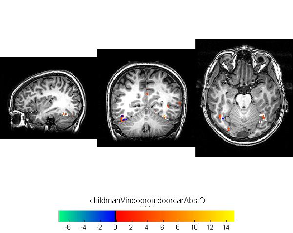
Below is another example of a reinotopic map in a different subject.
Figure 2
Once you upload the images, they look like this. Note that you can control many features of the images, like whether to show a thumbnail, and the display resolution.

MNI space
MNI is an abbreviation for Montreal Neurological Institute.
Methods
Measuring retinotopic maps
Retinotopic maps were obtained in 5 subjects using Population Receptive Field mapping methods Dumoulin and Wandell (2008). These data were collected for another research project in the Wandell lab. We re-analyzed the data for this project, as described below.
Subjects
Subjects were 5 healthy volunteers.
MR acquisition
Data were obtained on a GE scanner. Et cetera.
MR Analysis
The MR data was analyzed using mrVista software tools.
Pre-processing
All data were slice-time corrected, motion corrected, and repeated scans were averaged together to create a single average scan for each subject. Et cetera.
PRF model fits
PRF models were fit with a 2-gaussian model.
MNI space
After a pRF model was solved for each subject, the model was trasnformed into MNI template space. This was done by first aligning the high resolution t1-weighted anatomical scan from each subject to an MNI template. Since the pRF model was coregistered to the t1-anatomical scan, the same alignment matrix could then be applied to the pRF model.
Once each pRF model was aligned to MNI space, 4 model parameters - x, y, sigma, and r^2 - were averaged across each of the 6 subjects in each voxel.
Et cetera.
Results - What you found
Retinotopic models in native space
Some text. Some analysis. Some figures.
Retinotopic models in individual subjects transformed into MNI space
Some text. Some analysis. Some figures.
Retinotopic models in group-averaged data on the MNI template brain
Some text. Some analysis. Some figures. Maybe some equations.
Equations
If you want to use equations, you can use the same formats that are use on wikipedia.
See wikimedia help on formulas for help.
This example of equation use is copied and pasted from wikipedia's article on the DFT.
The sequence of N complex numbers x0, ..., xN−1 is transformed into the sequence of N complex numbers X0, ..., XN−1 by the DFT according to the formula:
where i is the imaginary unit and is a primitive N'th root of unity. (This expression can also be written in terms of a DFT matrix; when scaled appropriately it becomes a unitary matrix and the Xk can thus be viewed as coefficients of x in an orthonormal basis.)
The transform is sometimes denoted by the symbol , as in or or .
The inverse discrete Fourier transform (IDFT) is given by
Retinotopic models in group-averaged data projected back into native space
Some text. Some analysis. Some figures.
Conclusions
Here is where you say what your results mean.
References
Software
Appendix I - Code and Data
Code
Data
Appendix II - Work partition (if a group project)
Brian and Bob gave the lectures. Jon mucked around on the wiki.
