2009 Blair Bohannan

Back to Psych 204 Projects 2009

Project Title - MATLAB image processing tutorial

This page accompanies a MATLAB tutorial which simulates some artifacts that might be found in MR images. Their causes, and in some cases corrections, are demonstrated in the code. One- and two-dimensional examples are provided.
Image artifacts in this tutorial include DC Offset, Quadrature Ghosting, RF Noise, Gradient, and Frequency-Sampling Jitter. Information on the first four topics can be found in Hornak, Joseph P. The Basics of MRI, Chapter 11. More information on the mathematical derivations can be found in Smith, Julius O. Mathematics of the Discrete Fourier Transform (DFT). These and other references are listed at the bottom of this page.

About the tutorial

This tutorial consists of a MATLAB (.m) script and some image files. Unzip the files to a folder and either add to path or set the MATLAB workspace to this folder before starting the tutorial.
The tutorial uses cells, and each section below corresponds to a cell in the tutorial. To evaluate a cell in the tutorial, first navigate into it. Ctrl+Enter evaluates the current cell, and Ctrl+Shift+Enter evaluates and moves to the next cell. Variables are re-used throughout the tutorial, so start at the first cell and work through the tutorial in order.
The tutorial package contains a selection of image files. The "brain.jpg" image is from a k-space tutorial that was included with the materials for this class. Those titled "stimulus##.tif" (including the one used on this page) are taken, with permission, from an image set prepared by Roozbeh Kiani. The associated publication can be found here.

About this page

This page contains a narrative description of the concepts covered in the tutorial, along with figures that are generated by running the tutorial. In general, code examples will not be included here, but the tutorial code can be downloaded in its entirety from Appendix I below.

Tutorial

Cell I. Loading images for analysis

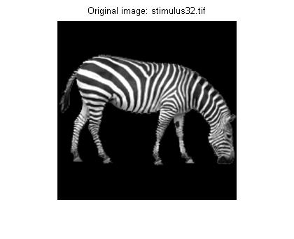
The first cell simply loads an image, converts it to grayscale, and sets the size of the image. nPix, the variable setting the number of pixels in the x and y dimensions, should be a power of 2 for faster FFT calculation.
This figure contains the image in grayscale. It has nPix x nPix pixels (in this case, 256 x 256).

Cell II. Using fftshift

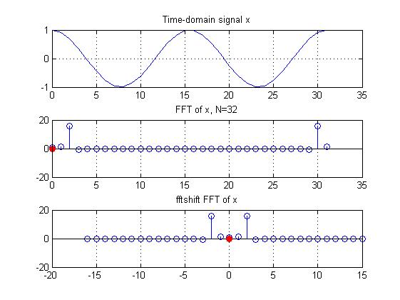
The fftshift function is helpful for visualizing Fourier transforms in a familiar format. (Note that for this tutorial we will be using the discrete Fourier transform.) In the 1-dimensional N-point Fourier transform (like the transform of an audio signal), it takes points N/2+1 to N (containing the Nyquist and negative frequency components) and moves them to the beginning of the array. See Oppenheim and Schafer, Chapter 4, if you want to know more about repeated spectrums due to sampling. Thus, the fftshifted function causes the positive and negative frequencies to be symmetric about the zero-frequency point. This being the case, it's helpful to keep in mind that the zero-frequency sample is at sample N/2+1.
Here is a 1-dimensional example. The red dot is the zero-frequency component of the transform of the sinusoid in the top subplot.

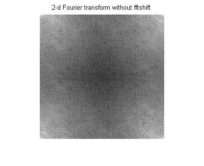
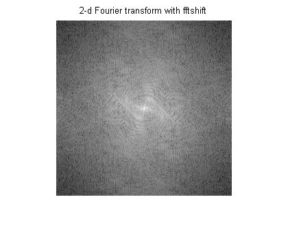
In the 2-dimensional case, fftshift swaps quadrants 1 and 3, and also 2 and 4 of the Fourier transform. Thus, the low-frequency information is moved to the center of the image, with the [0,0] frequency point moving from matrix index [1,1] to [nPix/2+1,nPix/2+1]. The fftshifted Fourier transform of an image is what we are used to looking at when we talk about k-space. For the purpose of this tutorial, time domain is the 1-dimensional case of image domain, and k-space is specifically the 2-dimensional case of frequency domain.
Here is a 2-d Fourier transform without fftshift. Note the bright spots (high amplitudes) in the outer corners of the image; these are the low frequencies.

Here is the same transform, with fftshift applied to it. Now the low-frequency, high-amplitude information is in the center of the image.
Note: fftshift should be used on the frequency-domain signal. Example:

X=fftshift(fft(x));

Using ifftshift

The ifftshift function reverses the effect of fftshift (use this instead of performing fftshift twice). Like fftshift, ifftshift is always applied to the frequency-domain signal in this tutorial, as follows:

x=ifft(ifftshift(X));

Cell III. Artifact 1: DC offset

Derivation

The DC offset is a constant, positive shift in amplitude. It results in a large peak at frequency zero. This can be derived from the equation for the DFT. Recall that the DFT is defined as

$X_{k}=\sum _{n=0}^{N-1}x_{n}e^{-{\frac {j2\pi }{N}}kn}\quad \quad k=0,\dots ,N-1$

where $x$ is the time signal at times $n$ and $X$ is the Fourier transform at frequency indices $k$. The DFT of a signal $x$ plus a constant DC offset $\Delta$ would then be

$X_{k}=\sum _{n=0}^{N-1}(x_{n}+\Delta )e^{-{\frac {j2\pi }{N}}kn}\quad \quad k=0,\dots ,N-1$

Since this is a linear system, we can separate the DC component from the original signal.

$X_{k}=\sum _{n=0}^{N-1}x_{n}e^{-{\frac {j2\pi }{N}}kn}+\sum _{n=0}^{N-1}\Delta _{n}e^{-{\frac {j2\pi }{N}}kn}\quad \quad k=0,\dots ,N-1$

We are interested in what is going on at frequency $k=0$. Assuming that the first term does not have some other DC artifact, we know that its zero-frequency component should be zero (this has to do with orthogonality of the DFT sinusoids). Focusing on the second term, since we are considering frequency $k=0$, the exponential is equal to $1$ for all $n$. Thus, the amplitude of the transform at this frequency is the sum of every term in the DC signal.

$X_{0}=N\Delta$

One-dimensional example

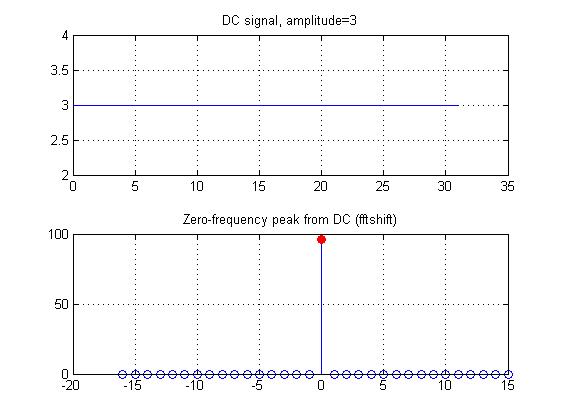
Here is a DC signal and its Fourier transform. Note that the DC amplitude is 3 and the FFT length is 32, making the zero-frequency peak 96.

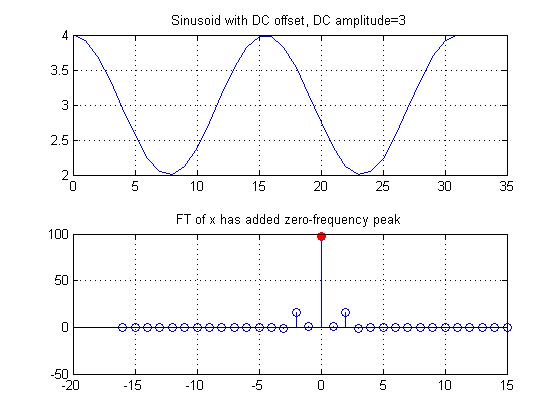
Here is the same DC signal added to the sinusoid from the previous section. Note that while the sinusoid was previously centered around 0, now it is centered around 3, the DC amplitude. The Fourier transform of this signal is the Fourier transform from before, with the added peak at zero.

Two-dimensional example

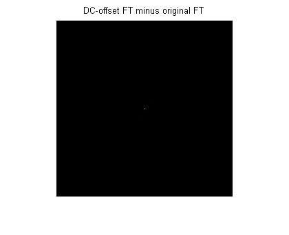
The same will be the case for 2-dimensional data. The image will have a bright spot in the center (at frequency [0,0]). In the next figure, the zebra image has been combined with a large DC offset and frequency transformed. The original Fourier transform has been subtracted from this artifact Fourier transform, and we are left with only the bright spot.

Cell IV. Removing time-domain DC offset

Two quick solutions come to mind for removing the time-domain (or image-domain) DC offset:

• Subtract the mean of the signal from every sample;
• Use a narrow highpass filter to remove the zero frequency component.

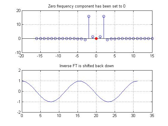
Here is the 1-dimensional example from the previous section. The zero-frequency component has simply been set to zero (so it has effectively been filtered out). The IFFT of this new transform has shifted the original signal back down.

Cell V. Frequency-domain DC offset

Derivation

DC offset can occur in the frequency domain as well, with similar effects. Note, however, that the equation for the IDFT contains a scaling factor ${\frac {1}{N}}$ before the summation:

$x_{n}={\frac {1}{N}}\sum _{k=0}^{N-1}X_{k}e^{{\frac {j2\pi }{N}}kn}\quad \quad n=0,\dots ,N-1$

(this would be ${\frac {1}{N^{2}}}$ for the 2-dimensional case)
Therefore, the peak at time $n=0$ will simply be the DC amplitude $\Delta$, not $N\Delta$.

One-dimensional example

Here is the frequency-domain offset for a 1-dimensional signal. The top subplot shows the sinusoid's Fourier transform, shifted up by a constant amount. The bottom subplot shows the inverse Fourier transform. The signal at time 0 now has the DC amplitude added to what was already present.

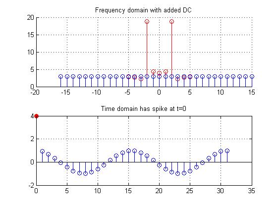
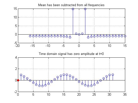
As in the time-domain case, this artifact can be removed by subtracting the mean of the Fourier transform from every element (in the Fourier transform). Note in the figure below, though, that doing so removes the entire signal at time zero, so the original signal at the time needs to be recovered (this can be done with some form of interpolation).

Cell VI. Frequency-domain DC offset - two-dimensional case

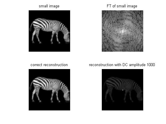
Here is an example of the effect of a k-space DC offset on a reconstructed image. The original zebra image has been reduced to a smaller pixel set so that the artifact is easier to see. The top two plots show the original image and its Fourier transform. The bottom two plots show the reconstruction of the original Fourier transform and the reconstruction of a Fourier transform that has a large DC offset. Note that the high amplitude of the bright spot has obscured the rest of the image.

Cell VII. Artifact 2: Quadrature ghost

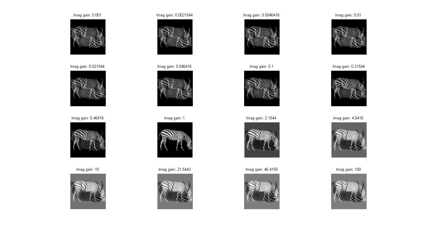
Another artifact discussed in the Hornak text, quadrature ghosting occurs when there is "a mismatch in the gain of the real and imaginary channels of the quadrature detector." [Hornak, Chapter 11]. It causes a shadow of the image to appear, rotated by 180 degrees. While this artifact was listed in the book, I've been told by the course instructors that it has become uncommon due to better equipment and oversampling during image acquisition.
In this figure, the imaginary gains have been varied systematically while the real gain is held constant. Note that the saturation changes in character depending on whether the imaginary gain is less than or greater than the real gain. As expected, the artifact is absent when the imaginary gain is equal to one.

Cell VIII. Artifact 3: RF noise

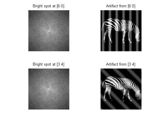
RF noise can cause amplitude spikes during image acquisition. A high-amplitude spike at a single pixel can cause a grating to become superimposed upon the reconstructed image. This grating will be oriented perpendicular to the vector drawn from the center of the image to the coordinates of the noisy pixel, and its frequency will be equal to the magnitude of that vector.
Here are two examples of such an event. In the top row, a noise spike at [6,0] from the origin has resulted in a vertical grating of frequency 6. In the bottom row, a noise spike at [3,4] has resulted in a diagonal grating of frequency 5 (the coordinates of this second case may need to be adjusted slightly to reach the exact frequency).

Cell IX. Systematic variation of frequency and rf noise amplitude

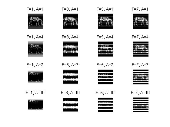
Here are more examples, with the frequency and amplitude scaling factor varied systematically. F is the frequency and A is the multiplicative amplitude increase.

Cell X. Adding rf noise to all pixels

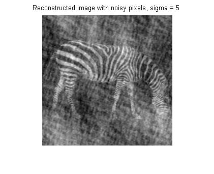
While adding a single, high-amplitude noise spike is helpful to demonstrate this artifact, it is probably more likely that small amounts of noise will be present in all of the k-space pixels. We can simulate this effect by creating a matrix of noise by which the original k-space matrix will be multiplied. A multiplicative rather than an additive matrix is being used due to the large variation in amplitude, especially in the lower frequencies.
Here is an example with sigma, the scaling factor, set to 5.

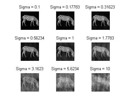
Below, sigma is varied systematically.

Cell XI. Artifact 4: Gradient

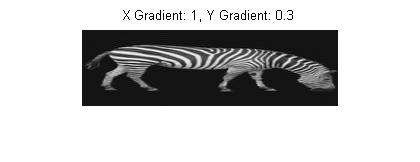
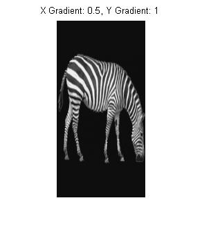
The gradient artifact occurs if the sampling frequency on either axis has been truncated. Hornak describes this as one of the gradients "operating at half of its expected value" (any other fractional increment could work as well).
Here are two examples of gradient error. The "X gradient" and "Y gradient" values indicate at what fraction of its expected value each axis's gradient is operating.

Cell XII. Artifact 5: Sampling jitter

The final artifact presented in the tutorial involves the effect of jitter. For MR imaging purposes, this refers to the image being acquired (sampled) at frequencies that differ by small amounts from the expected integer frequencies. Rather than being sampled at frequencies $1,2,\dots$, it may have in fact been sampled at frequencies $1+\delta _{1},2+\delta _{2},\dots$, where the $\delta$ values refer to small offsets (like -0.1, 0.05, etc). This will cause problems during image reconstruction as the ifft function does not know that the image was sampled at these non-integer frequencies, and evaluates each sample as though it were on an integer index.

One-dimensional time-domain example

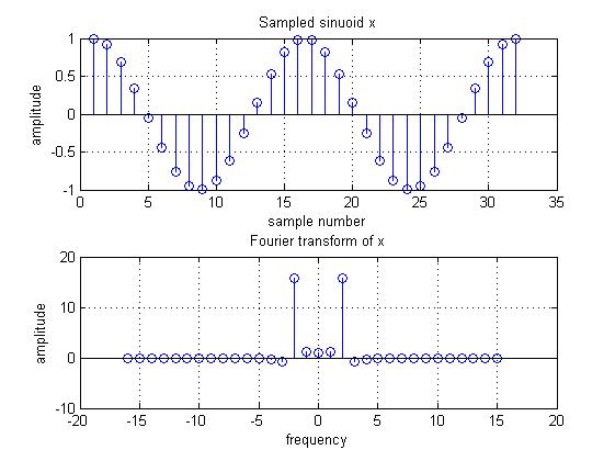
Here is the sinusoid from earlier, and its Fourier transform. The time index starts from 1.

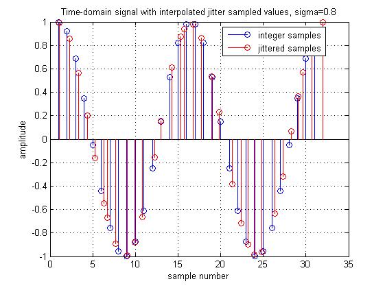
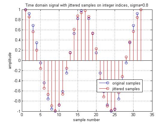
What happens to the Fourier transform if this time-domain signal is not sampled at the exact integer increments? We can add some jitter to the time indices and sample the interpolated signal at those points, then force these samples into the integer indices and see what happens.
The interp1 function can accomplish this. For our purposes, it will take in the original input vector (time-index integers), original output vector (the sinusoid), and the modified input vector (jittered time indices), outputting the sinusoid values at those jittered time indices.
In the figure below, we can see the original sinusoid (in blue) and the sinusoid at the jittered time values (in red). The jittered samples are being displayed at the time points at which they were sampled, which is why the shape of the sinusoid still looks normal.

The FFT will assume, though, that these red values were sampled on the integer time indices. This figure shows the effective signal whose FFT will be taken. Each red sample from the previous figure has been shifted in time onto its respective integer index. The resulting signal is a slightly distorted version of the original sinusoid.

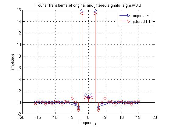
The resulting Fourier transforms are shown in the next figure. The correct (original) one is in blue; note the way that the jittered FT (in red) deviates slightly.

Cell XIII. Frequency-domain jitter

Two-dimensional example

It will be a similar situation for jitter in the frequency domain, and also for 2-dimensional signals.
This can be simulated in the same way as the 1-dimensional signal, except with the interp2 function. This function takes in two extra inputs, as the coordinates and jittered coordinates are specified for the x and y dimensions separately. The Fourier transform of the zebra image can be modified (in the frequency, or k-space, domain) in the same way the 1-dimensional signal was modified previously.
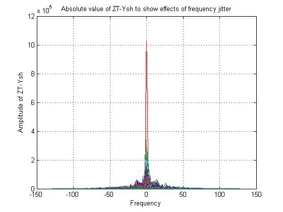
Here is a plot of the difference in the original and jittered Fourier transforms. Given that low-frequency components have the highest amplitude, it makes sense that the frequencies in the center are most sensitive to frequency sampling error.

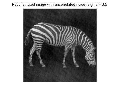
And here is the reconstructed image from the jittered Fourier transform.

Cell XIV. Correlating noise values for frequency jitter

The previous section used uncorrelated frequency shifts. It may be more realistic to suppose that in signal acquisition, these shifts will be more correlated to each other. This can be simulated by lowpass filtering the noise values to extract low-frequency periodicity.

Here is an example. The top subplot contains uncorrelated noise - the kind that was used for the simulation in the previous section. The bottom subplot shows the same noise, lowpass filtered with a cutoff frequency of 0.02.

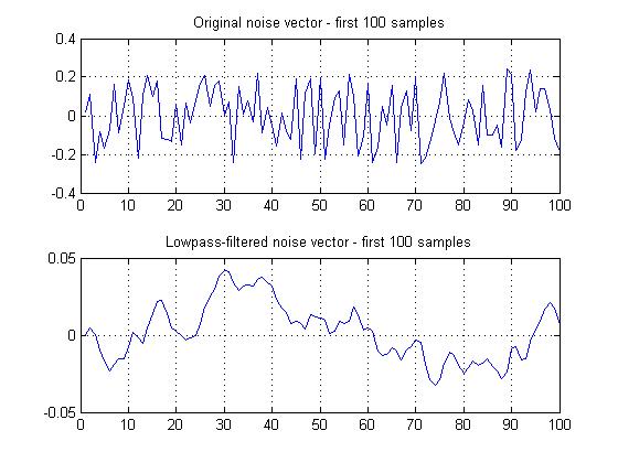
Note, though, that the amplitude of the filtered noise has dropped considerably. We can scale it back up, achieving the result found in Figure 26. Keep in mind that this figure plots only the first 100 samples, so the highest-amplitude sample might not be displayed.

Here is the reconstructed image with this random-walk noise. The noise is harder to detect; is is also more concentrated around the figure of the zebra.

Cell XV. Effect of sigma on frequency jitter

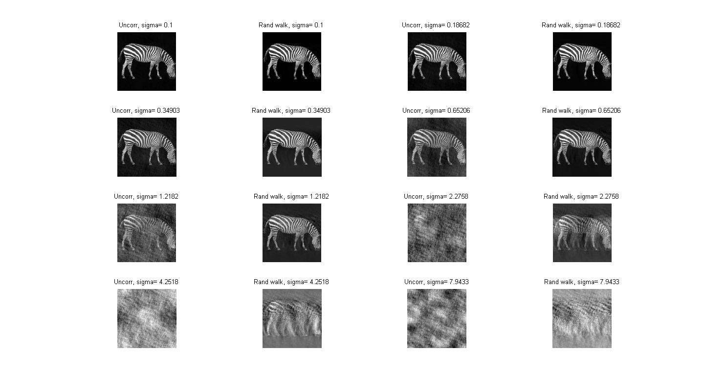
Finally, the effects of varying sigma (range of jitter) are shown for both uncorrelated and random-walk noise.

Appendix 1: Code

imageProcessing.zip

Appendix 2: Acknowledgements

I received help from Jonathan Abel (Consulting Professor, CCRMA) with some of the derivations, and also with the conceptualization of implementing the jitter artifact.
The Psych 204 instructors and TA offered helpful and practical suggestions toward improving and expanding the tutorial. Thank you!

References/Further reading

Huettel, Scott A., Andrew W. Song, and Gregory McCarthy. Functional Magnetic Resonance Imaging, 2nd Edition. Sunderland, Massachusetts: Sinauer Associates, 2009.
Hornak, Joseph P. The Basics of MRI.
Kiani, R., Esteky, H., Mirpour, K., and Tanaka, K. (2007). Object category structure in response patterns of neuronal population in monkey inferior temporal cortex. J. Neurophysiol. 97, 4296–4309. pdf
Oppenheim, Alan V., and Ronald W. Schafer. Discrete-Time Signal Processing, 2nd Edition. Prentice Hall Signal Processing Series. Upper Saddle River, New Jersey: Prentice Hall, 1999.
Smith, Julius O. Mathematics of the Discrete Fourier Transform (DFT) with Audio Applications, 2nd Edition. W3K Publishing, 2007.