Mai

This page describes the traveling wave model of retinotopy with as little math as possible, providing a hopefully more intuitive understanding of phase-encoding. For people unfamiliar with the Fourier Transform or are mathematically inept (like myself), I have a second page, Fourier transform math , that goes through some of the math involved.

Introduction to retinotopy

Early visual areas, located in the posterior occipital lobe, are retinotopically organized: A particular location in the early visual cortex responds to stimulation at a particular location in the visual field, while neighboring locations on the cortical surface respond to neighboring locations in the visual field. This pattern of response maps a representation of the visual field onto the cortical surface.

Retinotopic areas on example subject

These early visual areas are mapped with two parameters: eccentricity and polar angle. Eccentricity indicates distance from fovea. The most posterior regions of the early visual areas has a pronounced foveal preference, while more anterior regions prefer more eccentric stimuli. In visualizations of retinotopy, eccentricity mapping appears as concentric "rings" of different colors, each denoting a different eccentricity. Polar angle indicates the angle from the horizontal meridian, so polar angle mapping shows the reversals in angular representations on the cortex, which are used in defining retinotopic maps.

While the primary visual cortex (V1) was the first visual field map discovered, over the last 15 years, a variety of retinotopic maps have been identified on the ventral and dorsal surface of visual cortex. While definitions of these visual areas will not be discussed, more information about these retinotopic maps can be found here. Information about defining these regions can be found here and here.

Traveling wave model

Stimuli used in mapping polar angle (top) and eccentricity (bottom)

While retinotopic maps were first identified in the 1940s ago using electrophysiology, it is only in the last 20 years that these maps have been identified using fMRI. The turning point was in 1994 when Engel, Glover, and Wandell developed a new method for mapping visual field maps using a "traveling wave" of activation. First used to map eccentricity in V1, this method was a vast improvement on previous methods. In a nutshell, this method activates different regions of the visual cortex at different times, creating a "traveling wave" of activation from one region to another. The delay in activation allows us to infer the eccentricity or polar angle preference of a region. So how does this actually work?

The Stimuli

Early visual cortex has both eccentricity and polar angle mapping, so two types of stimuli are needed. Eccentricity is mapped using a series of expanding, concentric checkerboard rings while polar angle is mapped by a rotating checkerboard wedge. These checkerboard patterns have been demonstrated to generate a strong neural response in early visual areas.

These stimuli are designed to activate adjacent retinotopic voxels sequentially, such that voxels with different eccentricity (or polar angle) preferences are activated at different times. For example, let's consider a hypothetical row of retinotopic voxels along the calcarine sulcus, from posterior to anterior:

We know the most posterior voxels (the two boxes furthest to the left) have a foveal preference. In an eccentricity experiment with a expanding series of rings, these voxels will therefore be activated really early on (t = 0, hypothetically). The two voxels in the middle are more anterior, so they probably have a more peripheral preference relative to the first two voxels, so they won't be activated until later in time. The most anterior voxels with the most peripheral preference will be activated last in time, so there is a "traveling wave" of activation from posterior to anterior (thus the name "traveling wave model").

This seems like a really simple idea, but it's absolutely critical to understanding the traveling wave model.

• More posterior voxels are activated first
• Most anterior voxels are activated later

Phase Encoding

The traveling wave of activation created by the stimuli means that we can extract (in this case) eccentricity preference from the time series for a retinotopic voxel.

Let's think about the hypothetical time series for a hypothetical retinotopic voxel:

This time series has 6 peaks because a typical retinotopic scan has 6 cycles of the stimulus. More importantly, we see that the signal starts rising at t = 0. This hypothetical voxel must have been activated very early in the cycle, which means that it was probably activated by a foveal stimulus--so this voxel probably has a foveal preference.

In contrast, let's look at another hypothetical time series, that is almost identical to the one above:

Like the first time series, this one also has 6 peaks--but there's a delay before the signal begins rising. It is "phase-shifted" to the right, which just means that this voxel was activated later in time relative to the first one. If it was activated later in time, it was probably activated by a more peripheral stimulus, so this voxel probably has a peripheral preference. Thus, voxels activated later in time are "phase shifted," so the location preference for a voxel is "phase encoded." Given a voxel time series, we can find its eccentricity (or polar angle) preference by determining its phase.

Finding the phase

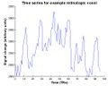
In practice of course, the time series for a retinotopic voxel never looks that nice. To the right is the unfiltered time series for a real voxel. While the six peaks corresponding to the six cycles of the experiment are readily apparent, there is still a significant amount of noise from signal drift, thermal noise, and physiological noise. This scan has already been motion corrected.

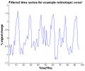
Thus, before this voxel's phase can be determined, the time series needs to be filtered to remove noise. Here, the time series was detrended by removing the baseline and then dividing by the mean signal. The resulting filtered time series still has the six peaks, but the most obvious noise has been removed so that the peaks are varying around 0. Now we can think about finding the phase, and therefore location preference.

• 

  raw time series

• 

  filtered time series

The "best fitting" sine wave

To find the phase of the filtered time series, we need to find the sine wave that best explains the time series. This "best fitting" sine wave will have peaks where the time series has peaks and troughs where the time series has troughs, or essentially a high correlation between the sine wave and the time series. In math speak, this sine wave can be written as:

sine wave = amplitude * sin(2*pi * frequency - phase)

• frequency is just the number of times the sine wave repeats
• phase is the time shift we're looking for
• amplitude stretches the sine wave up and down. More precisely, the amplitude is a measure of the "power" of this sine wave, or how much this sine wave overlaps with the time series. A large amplitude indicates high power, or a high overlap.

Finding this "best fitting" sine wave is more complicated than it might seem, so we'll need to take a short mathematical digression.

Discrete Fourier Transform

Any signal can be written as the sum of sine waves at different frequencies.

• • These frequencies range from 0 to #TRs/2 (in our case 96/2 = 48), so the time series can be written as the sum of 48 different sine waves
    • The #TRs/2 is the Nyquist frequency, which sets the maximum resolution for a discretely sampled signal. Using frequencies > #TRs/2 will result in aliasing.
  • Each of these 48 sine waves will have a different amplitude and phase
    • Amplitude = measure of "power" or how much a sine wave at a particular frequency describes the time series
    • Phase = time shift to the right

The Fourier transform lets us find the phase and amplitude for each of these 48 sine waves at different frequencies. The sine wave that best explains the time series is the sine wave with the largest amplitude. The phase of the time series is the phase of this best fitting sine wave.

Sine wave at stimulus frequency

By taking the Fourier transform at every frequency from 0 to #TRs/2, we can build up a frequency spectrum. This spectrum plots the amplitude of each sine wave at all of the frequencies. It is also sometimes called a power spectrum, since it shows the power (which is just amplitude) of each frequency in describing the original time series.

The spectrum shows that the sine wave at the stimulus frequency (6 cycles/scan) has the largest amplitude, or the most power in describing the time series. This sine wave has peaks were the time series has peaks, and troughs where the time series has troughs. Thus, the phase of this sine wave describes the phase of the time series, allowing us to extract location preference for this voxel.

Build visual area map

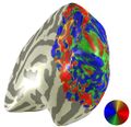
Repeating the above analysis for every voxel produces a visualization of the retinotopic maps. However, a major problem of this analysis is that the Fourier transform will return a phase and amplitude at the stimulus frequency for every single voxel--even ones that are not retinotopic. For example, the polar angle map on the right hemisphere of subject LM (on right) shows a lot of noise from non-retinotopic voxels. More anterior voxels or voxels with that prefer stimuli from the right half of the visual field (tan voxels) are probably not retinotopic, so we need a method to filter these voxels out.

• 

  unthresholded polar angle map on adult LM

• 

  threshold at coherence = .2

If we look at the frequency spectrum of retinotopic voxels, we will see a large peak at the stimulus frequency (6 cycles/scan), as we saw earlier for the example retinotopic voxe. This large peak indicates that the sine wave at the stimulus frequency describes the voxel's time series really well, which is what we would expect. A non-retinotopic voxel, in contrast, would not have a large peak at the stimulus frequency. A non retinotopic voxel is not activated by the stimulus, so its time series should just show random noise that doesn't correlate with the stimulus. Thus, a good way of filtering out non-retinotopic voxels might be to look at the voxel's amplitude at the stimulus frequency relative to the total power in the spectrum. This measure is called "coherence," and can be thought of as a measure of variance explained. Typically, we threshold to a coherence level of around 0.20.

References

• Engel, S.A., Rumelhart, D.E., Wandell, B.A., Lee, A.T., Glover, G.H., Chichilnisky, E.J., & Shadien, M.N. (1994). fMRI of human visual cortex. Nature, 369: 525.
• Engel, S.A., Glover, G.H., & Wandell, B.A. (1997). Retinotopic organization in human visual cortex and the spatial precision of functional MRI. Cerebral Cortex, 7: 181-192.
• Engel, S.A. (2011). The development and use of phase-encoded functional MRI designs. Neuroimage.
• Wandell, B.A. (1999). Computational neuroimaging of human visual cortex. Annual Reviews Neuroscience," 22: 145-73.
• Wandell, B.A., Brewer, A.A., & Dougherty, A.A. (2005). Visual field map clusters in human cortex. Philosophical transactions of the royal society, 360: 693-707.
• Wandell, B.A., Dumoulin, S.O., & Brewer, A.A. (2007). Visual field maps in human cortex. Neuron, 56: 366-383.